KeplerSystem’s other perturbation: the power-law term

Kepler orbits and perihelion precession shows apsidal precession from the effective post-Newtonian \(c_\mathrm{pn}/r^3\) correction. KeplerSystem has a second, independent perturbation family added to its radial potential:

\[V(r) = -\frac{k}{r} + \frac{c_\varepsilon}{r^{1+\varepsilon}} ,\]

an adjustable power-law addition to the pure \(1/r\) potential. At \(\varepsilon=0\) this is degenerate – it is just another \(1/r\) term, rescaling the effective coupling constant, so by Bertrand’s theorem the orbit stays a perfectly closed, non-precessing ellipse. For any \(\varepsilon \neq 0\), Bertrand’s theorem no longer applies and the orbit precesses, faster for larger \(\varepsilon\) – shown here for three exponents at the same coefficient, all still exactly energy-conserving.

import matplotlib.pyplot as plt
import numpy as np

from physicskit.classical.systems.newtonian import KeplerSystem

fig, axes = plt.subplots(1, 3, figsize=(13, 4.3))
for ax, eps in zip(axes, (0.5, 1.0, 2.0)):
    system = KeplerSystem.from_orbital_elements(a=1.0, e=0.4, eps=eps, c_eps=0.01)
    lrl0 = system.lrl_vector()
    result = system.integrate((0, 100), dt=1e-3, method="yoshida4")

    lrl_vecs = np.array([system.lrl_vector(q, p) for q, p in zip(result.q, result.p)])
    angle = np.arctan2(lrl_vecs[:, 1], lrl_vecs[:, 0]) - np.arctan2(lrl0[1], lrl0[0])
    drift = np.max(np.abs(result.energy - result.energy[0])) / abs(result.energy[0])
    print(f"eps={eps}: precession over t=100 = {np.unwrap(angle)[-1]:+.3f} rad, energy drift = {drift:.2e}")

    ax.plot(result.q[:, 0], result.q[:, 1], color="steelblue", lw=0.6)
    ax.plot(0, 0, "o", color="gold")
    ax.set_title(f"eps = {eps}")
    ax.set_aspect("equal")
fig.suptitle(r"$V(r) = -k/r + c_\varepsilon / r^{1+\varepsilon}$: precession grows with $\varepsilon$", fontsize=13)
fig.tight_layout(rect=[0, 0, 1, 0.92])

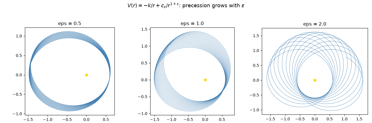
eps=0.5: precession over t=100 = -0.362 rad, energy drift = 5.71e-12
eps=1.0: precession over t=100 = -1.057 rad, energy drift = 5.71e-12
eps=2.0: precession over t=100 = -3.237 rad, energy drift = 5.05e-12

See Angular momentum: a different conservation law from energy for a related point: even with this perturbation switched on, the orbit’s angular momentum – a different conserved quantity from energy – stays exactly constant, since V(r) depends only on r and the force therefore still exerts no torque about the origin.

plt.show()