The intermediate axis theorem (Dzhanibekov effect)

EulerTop is a torque-free rigid body: Euler’s equations for the body-frame angular velocity \(\boldsymbol\omega = (\omega_1, \omega_2, \omega_3)\) about the three principal axes, with moments of inertia \(I_1, I_2, I_3\),

\[I_1\dot\omega_1 = (I_2 - I_3)\,\omega_2\omega_3, \qquad I_2\dot\omega_2 = (I_3 - I_1)\,\omega_3\omega_1, \qquad I_3\dot\omega_3 = (I_1 - I_2)\,\omega_1\omega_2 ,\]

coupled to the orientation quaternion. Spin a rigid body about its largest- or smallest-moment-of-inertia axis and it spins smoothly forever; spin it about the intermediate axis and it tumbles periodically – the intermediate axis theorem, popularized as the “Dzhanibekov effect.” EulerTop integrates these equations with implicit_midpoint, which exactly conserves every quadratic invariant of the combined state (rotational kinetic energy \(\tfrac12\sum_i I_i\omega_i^2\), \(|L|^2 = \sum_i (I_i\omega_i)^2\), quaternion norm) regardless of how non-linear the tumbling dynamics is.

import matplotlib.pyplot as plt

from physicskit.classical.systems.rotations import EulerTop
from physicskit.classical.visualizers.phase_space import plot_so3_momentum_sphere

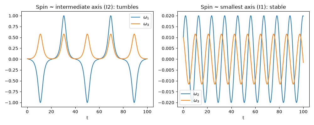
Tumbling (intermediate axis) vs. stable (smallest axis)

unstable = EulerTop(omega0=[0.01, 1.0, 0.01], I1=1.0, I2=2.0, I3=3.0)
stable = EulerTop(omega0=[1.0, 0.01, 0.01], I1=1.0, I2=2.0, I3=3.0)

r_unstable = unstable.integrate((0, 100), dt=1e-3, method="implicit_midpoint")
r_stable = stable.integrate((0, 100), dt=1e-3, method="implicit_midpoint")

E0 = unstable.energy()
L0 = unstable.angular_momentum_squared()
E_final = unstable.energy(r_unstable.y[-1])
L_final = unstable.angular_momentum_squared(r_unstable.y[-1])
print(f"energy drift: {abs(E_final - E0) / E0:.3e}, |L|^2 drift: {abs(L_final - L0) / L0:.3e}")

fig1, axes = plt.subplots(1, 2, figsize=(10, 4), sharex=True)
axes[0].plot(r_unstable.t, r_unstable.y[:, 0], label=r"$\omega_1$")
axes[0].plot(r_unstable.t, r_unstable.y[:, 2], label=r"$\omega_3$")
axes[0].set_title("Spin ~ intermediate axis (I2): tumbles")
axes[0].set_xlabel("t")
axes[0].legend()

axes[1].plot(r_stable.t, r_stable.y[:, 1], label=r"$\omega_2$")
axes[1].plot(r_stable.t, r_stable.y[:, 2], label=r"$\omega_3$")
axes[1].set_title("Spin ~ smallest axis (I1): stable")
axes[1].set_xlabel("t")
axes[1].legend()
fig1.tight_layout()

energy drift: 0.000e+00, |L|^2 drift: 0.000e+00

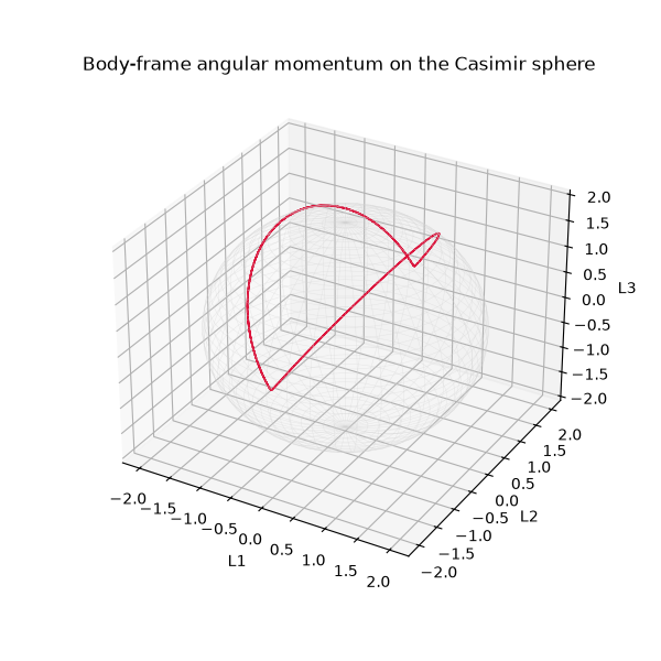
The polhode on the Casimir sphere

See The Dzhanibekov effect, literally: a tumbling 3D rigid body for an animation of the actual tumbling rigid body corresponding to this trajectory.

fig2 = plt.figure(figsize=(6, 6))
ax2 = fig2.add_subplot(111, projection="3d")
plot_so3_momentum_sphere(r_unstable.y[:, :3], I1=1.0, I2=2.0, I3=3.0, ax=ax2)

plt.show()