The heavy symmetric top: effective potential, precession and nutation

HeavySymmetricTop is a symmetric top with one point fixed, spinning under gravity, with generalized coordinates \(q = (\phi, \theta, \psi)\) – the standard z-x-z Euler angles (precession, nutation, spin) – and Lagrangian

\[L = \frac{I_1}{2}\left(\dot\theta^2 + \dot\phi^2\sin^2\theta\right) + \frac{I_3}{2}\left(\dot\psi + \dot\phi\cos\theta\right)^2 - M g l \cos\theta ,\]

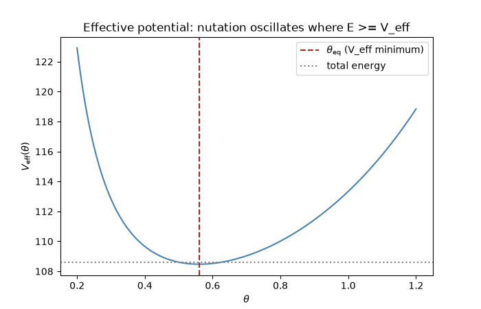
where \(I_1\) is the transverse moment of inertia about the fixed point, \(I_3\) the axial moment, \(M\) the mass, and \(l\) the pivot-to-center-of-mass distance. Because \(\phi\) and \(\psi\) are cyclic, their conjugate momenta \(p_\phi, p_\psi\) are conserved, and the dynamics of \(\theta\) alone reduce to 1-DOF motion in the effective potential

\[V_\mathrm{eff}(\theta) = \frac{(p_\phi - p_\psi\cos\theta)^2} {2 I_1 \sin^2\theta} + \frac{p_\psi^2}{2 I_3} + M g l \cos\theta ,\]

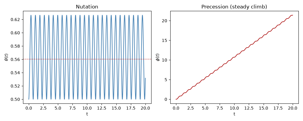
which governs the top’s nutation (the wobble in the tilt angle \(\theta\)), while \(\phi\) precesses steadily around it. This plots \(V_\mathrm{eff}\), integrates the top, and validates the closed-form/harmonic nutation and precession frequencies (nutation_frequency, precession_frequency) against an FFT of the actual trajectory.

import matplotlib.pyplot as plt
import numpy as np

from physicskit.classical.systems.rotations import (
    HeavySymmetricTop,
    effective_potential_symmetric_top,
    find_theta_equilibrium,
    nutation_frequency,
    precession_frequency,
)

I1, I3, M, l, g = 1.0, 0.5, 1.0, 1.0, 9.81
top = HeavySymmetricTop([0.0, 0.5, 0.0], [0.0, 0.0, 20.0], I1=I1, I3=I3, M=M, l=l, g=g)
p_phi, _, p_psi = top.momentum(top.q, top.qdot)

theta_eq = find_theta_equilibrium(p_phi, p_psi, I1, I3, M * g * l)
predicted_nutation = nutation_frequency(p_phi, p_psi, I1, I3, M * g * l, theta_eq=theta_eq)
predicted_precession = precession_frequency(p_phi, p_psi, I1, theta_eq)
print(f"theta_eq (V_eff minimum): {theta_eq:.4f} rad (started at theta0=0.5)")
print(f"predicted nutation frequency: {predicted_nutation:.4f} rad/s")
print(f"predicted precession frequency: {predicted_precession:.4f} rad/s")

result = top.integrate((0, 20.0), dt=2e-5, method="implicit_midpoint")

# FFT-measured nutation frequency and mean precession rate, for comparison.
theta_t = result.q[:, 1]
dt = result.t[1] - result.t[0]
spectrum = np.abs(np.fft.rfft(theta_t - theta_t.mean()))
freqs = np.fft.rfftfreq(len(theta_t), d=dt) * 2 * np.pi
measured_nutation = freqs[np.argmax(spectrum[1:]) + 1]
measured_precession = (result.q[-1, 0] - result.q[0, 0]) / (result.t[-1] - result.t[0])
print(f"measured nutation frequency (FFT peak): {measured_nutation:.4f} rad/s")
print(f"measured mean precession rate: {measured_precession:.4f} rad/s")

theta_eq (V_eff minimum): 0.5603 rad (started at theta0=0.5)
predicted nutation frequency: 8.1908 rad/s
predicted precession frequency: 1.0798 rad/s
measured nutation frequency (FFT peak): 8.1681 rad/s
measured mean precession rate: 1.0695 rad/s

Effective potential and where this top actually sits

theta_range = np.linspace(0.2, 1.2, 400)
veff = effective_potential_symmetric_top(theta_range, p_phi, p_psi, I1, I3, M * g * l)

fig1, ax = plt.subplots(figsize=(7, 4.5))
ax.plot(theta_range, veff, color="steelblue")
ax.axvline(theta_eq, color="firebrick", ls="--", label=r"$\theta_\mathrm{eq}$ (V_eff minimum)")
ax.axhline(top.energy(), color="0.5", ls=":", label="total energy")
ax.set_xlabel(r"$\theta$")
ax.set_ylabel(r"$V_\mathrm{eff}(\theta)$")
ax.set_title("Effective potential: nutation oscillates where E >= V_eff")
ax.legend()

<matplotlib.legend.Legend object at 0x36e28ef90>

Nutation (theta) and precession (phi) over time

fig2, axes = plt.subplots(1, 2, figsize=(10, 4))
axes[0].plot(result.t, result.q[:, 1], color="steelblue")
axes[0].axhline(theta_eq, color="firebrick", ls="--", lw=0.8)
axes[0].set_xlabel("t")
axes[0].set_ylabel(r"$\theta(t)$")
axes[0].set_title("Nutation")

axes[1].plot(result.t, result.q[:, 0], color="firebrick")
axes[1].set_xlabel("t")
axes[1].set_ylabel(r"$\phi(t)$")
axes[1].set_title("Precession (steady climb)")
fig2.tight_layout()

plt.show()