Born and von Karman: phonon dispersion of crystal lattices

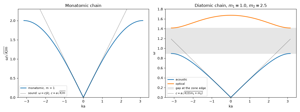
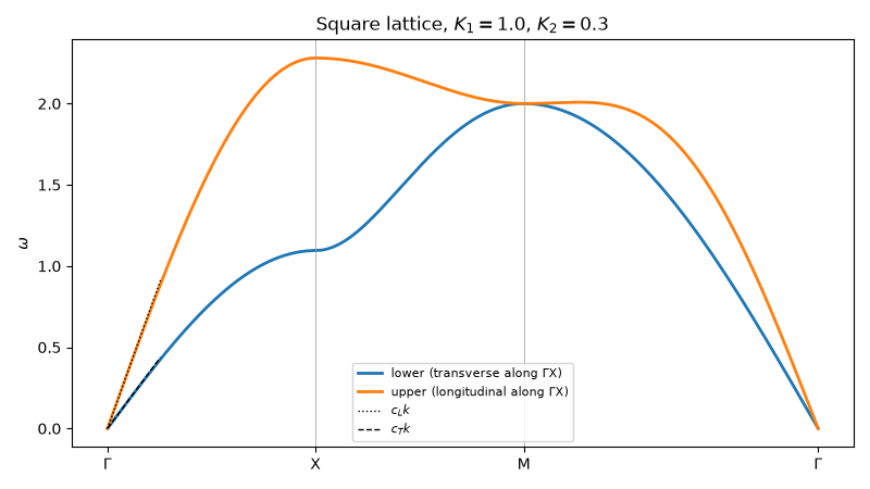
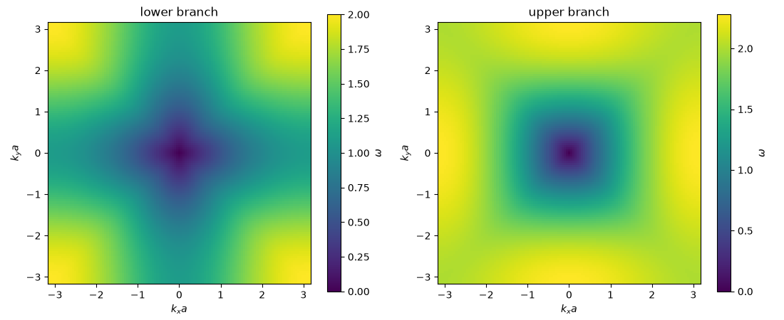
Born and von Karman (1912) treated a crystal as masses joined by springs with periodic boundary conditions, so that its vibrations are plane waves with a dispersion relation \(\omega(\mathbf k)\). This example shows the monatomic chain (monatomic_chain_dispersion()), the diatomic chain with its acoustic and optical branches and zone-boundary gap (diatomic_chain_dispersion()), and a 2D square lattice (square_lattice_phonon_dispersion()) whose acoustic branches start linearly with the sound speeds \(c_L = a\sqrt{(K_1+K_2)/m}\) and \(c_T = a\sqrt{K_2/m}\).

import matplotlib.pyplot as plt
import numpy as np

from physicskit.condensed.phonons import (
    diatomic_chain_dispersion,
    monatomic_chain_dispersion,
    square_lattice_phonon_dispersion,
)

One-dimensional chains

k = np.linspace(-np.pi, np.pi, 400)
K, m1, m2 = 1.0, 1.0, 2.5
ac, op = diatomic_chain_dispersion(k, K, m1, m2, a=1.0)

fig, axes = plt.subplots(1, 2, figsize=(12, 4.5))
axes[0].plot(k, monatomic_chain_dispersion(k, K, 1.0), lw=2, label="monatomic, m = 1")
axes[0].plot(k, np.abs(k), "k:", lw=1, label=r"sound: $\omega = c|k|$, $c = a\sqrt{K/m}$")
axes[0].set_ylim(0, 2.3)
axes[0].set_xlabel("ka")
axes[0].set_ylabel(r"$\omega / \sqrt{K/m}$")
axes[0].set_title("Monatomic chain")
axes[0].legend(fontsize=8)

axes[1].plot(k, ac, lw=2, label="acoustic")
axes[1].plot(k, op, lw=2, label="optical")
axes[1].axhspan(np.sqrt(2 * K / m2), np.sqrt(2 * K / m1), color="0.9", label="gap at the zone edge")
c_ac = np.sqrt(K / (2 * (m1 + m2)))
axes[1].plot(k, c_ac * np.abs(k), "k:", lw=1, label=r"$c = a\sqrt{K/2(m_1+m_2)}$")
axes[1].set_ylim(0, 1.8)
axes[1].set_xlabel("ka")
axes[1].set_ylabel(r"$\omega$")
axes[1].set_title(f"Diatomic chain, $m_1 = {m1}$, $m_2 = {m2}$")
axes[1].legend(fontsize=8)
fig.tight_layout()

The square lattice along a high-symmetry path

\(\Gamma = (0,0) \to X = (\pi,0) \to M = (\pi,\pi) \to \Gamma\). Next-nearest-neighbor springs \(K_2\) give the lattice its shear stiffness, and so the transverse branch.

K1, K2 = 1.0, 0.3
n = 150
path = np.concatenate(
    [
        np.column_stack([np.linspace(0, np.pi, n), np.zeros(n)]),
        np.column_stack([np.full(n, np.pi), np.linspace(0, np.pi, n)]),
        np.column_stack([np.linspace(np.pi, 0, n), np.linspace(np.pi, 0, n)]),
    ]
)
omega = square_lattice_phonon_dispersion(path[:, 0], path[:, 1], K1, K2)
s = np.concatenate([[0], np.cumsum(np.linalg.norm(np.diff(path, axis=0), axis=1))])

fig2, ax2 = plt.subplots(figsize=(8, 4.5))
ax2.plot(s, omega[:, 0], lw=2, label="lower (transverse along ΓX)")
ax2.plot(s, omega[:, 1], lw=2, label="upper (longitudinal along ΓX)")
kk = np.linspace(0, 0.8, 20)
ax2.plot(kk, np.sqrt(K1 + K2) * kk, "k:", lw=1, label=r"$c_L k$")
ax2.plot(kk, np.sqrt(K2) * kk, "k--", lw=1, label=r"$c_T k$")
for x in (s[n - 1], s[2 * n - 1]):
    ax2.axvline(x, color="0.6", lw=0.5)
ax2.set_xticks([0, s[n - 1], s[2 * n - 1], s[-1]], ["Γ", "X", "M", "Γ"])
ax2.set_ylabel(r"$\omega$")
ax2.set_title(rf"Square lattice, $K_1 = {K1}$, $K_2 = {K2}$")
ax2.legend(fontsize=8)
fig2.tight_layout()

Over the whole Brillouin zone

kx = np.linspace(-np.pi, np.pi, 121)
KX, KY = np.meshgrid(kx, kx)
w = square_lattice_phonon_dispersion(KX, KY, K1, K2)
fig3, axes3 = plt.subplots(1, 2, figsize=(11, 4.5))
for ax, branch, name in zip(axes3, (0, 1), ("lower", "upper")):
    im = ax.pcolormesh(KX, KY, w[..., branch], shading="auto", cmap="viridis")
    ax.set_aspect("equal")
    ax.set_xlabel(r"$k_x a$")
    ax.set_ylabel(r"$k_y a$")
    ax.set_title(f"{name} branch")
    fig3.colorbar(im, ax=ax, label=r"$\omega$")
fig3.tight_layout()

Check

Zone-edge gap of the diatomic chain: omega = sqrt(2K/m2), sqrt(2K/m1); sound speeds of the square lattice along Gamma-X: c_L = sqrt(K1 + K2), c_T = sqrt(K2).

edge = np.argmin(np.abs(k - np.pi))
assert np.isclose(ac[edge], np.sqrt(2 * K / m2), rtol=1e-4)
assert np.isclose(op[edge], np.sqrt(2 * K / m1), rtol=1e-4)
small = 3
np.testing.assert_allclose(omega[small] / path[small, 0], [np.sqrt(K2), np.sqrt(K1 + K2)], rtol=1e-3)