Debye’s heat capacity and the T³ law

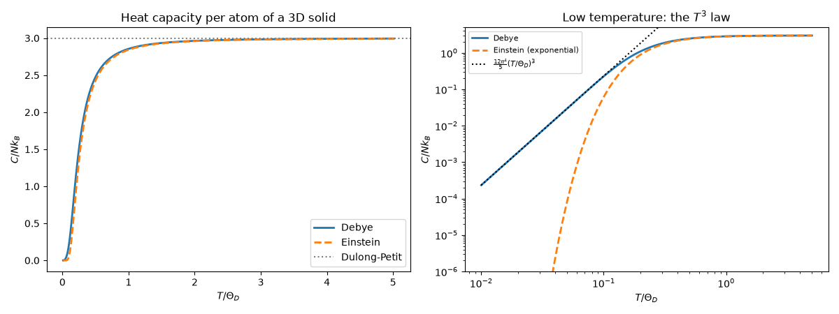
Einstein’s 1907 model, with every atom vibrating at one frequency, explained why heat capacities drop below the classical Dulong-Petit value \(3Nk_B\) at low temperature, but it predicted an exponential drop. Measurements showed a power law. Debye (1912) replaced the single frequency by sound waves with \(\omega = ck\) up to a cutoff \(\Theta_D\) and found \(C \approx \frac{12\pi^4}{5}Nk_B(T/\Theta_D)^3\) at low \(T\). debye_heat_capacity() is compared here with the Einstein model and with the heat capacity of an actual lattice dispersion (lattice_heat_capacity()).

import matplotlib.pyplot as plt
import numpy as np

from physicskit.condensed.phonons import (
    debye_heat_capacity,
    lattice_heat_capacity,
    monatomic_chain_dispersion,
    square_lattice_phonon_dispersion,
)

theta_D = 1.0
T = np.logspace(-2, 0.7, 120)

Debye vs. Einstein

The Einstein curve uses the frequency \(\omega_E = 0.806\,\Theta_D\) that matches Debye at high temperature (equal second moments). Only Debye’s model follows the \(T^3\) law seen in experiments.

C_debye = debye_heat_capacity(T, theta_D)
C_einstein = 3 * lattice_heat_capacity(np.array([0.806 * theta_D]), T)

fig, axes = plt.subplots(1, 2, figsize=(12, 4.5))
axes[0].plot(T, C_debye, lw=2, label="Debye")
axes[0].plot(T, C_einstein, lw=2, ls="--", label="Einstein")
axes[0].axhline(3, color="0.5", ls=":", label="Dulong-Petit")
axes[0].set_xlabel(r"$T / \Theta_D$")
axes[0].set_ylabel(r"$C / N k_B$")
axes[0].set_title("Heat capacity per atom of a 3D solid")
axes[0].legend()

axes[1].loglog(T, C_debye, lw=2, label="Debye")
axes[1].loglog(T, C_einstein, lw=2, ls="--", label="Einstein (exponential)")
axes[1].loglog(T, 12 * np.pi**4 / 5 * T**3, "k:", label=r"$\frac{12\pi^4}{5}(T/\Theta_D)^3$")
axes[1].set_ylim(1e-6, 5)
axes[1].set_xlabel(r"$T / \Theta_D$")
axes[1].set_ylabel(r"$C / N k_B$")
axes[1].set_title(r"Low temperature: the $T^3$ law")
axes[1].legend(fontsize=8)
fig.tight_layout()

Dimensionality: \(T^d\) from real lattice dispersions

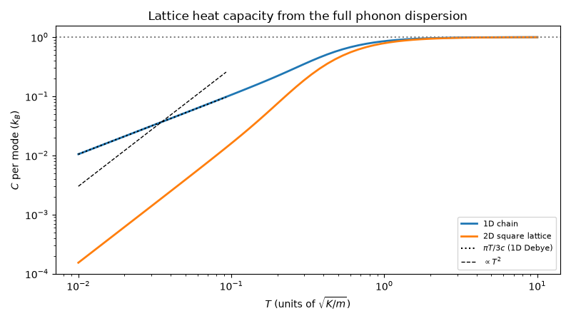
The power law comes from the acoustic phonons alone: a \(d\)-dimensional gas of linearly dispersing modes gives \(C \propto T^d\). Summing Einstein’s formula over the Brillouin zone of the 1D chain and the 2D square lattice gives \(T^1\) and \(T^2\).

k1 = 2 * np.pi * np.arange(20000) / 20000 - np.pi
w1 = monatomic_chain_dispersion(k1)
kk = 2 * np.pi * np.arange(300) / 300 - np.pi
KX, KY = np.meshgrid(kk, kk)
w2 = square_lattice_phonon_dispersion(KX, KY, 1.0, 0.5)

T_lat = np.logspace(-2, 1, 60)
fig2, ax2 = plt.subplots(figsize=(8, 4.5))
ax2.loglog(T_lat, lattice_heat_capacity(w1, T_lat), lw=2, label="1D chain")
ax2.loglog(T_lat, lattice_heat_capacity(w2, T_lat), lw=2, label="2D square lattice")
ax2.loglog(T_lat[:20], np.pi * T_lat[:20] / 3, "k:", label=r"$\pi T/3c$ (1D Debye)")
ax2.loglog(T_lat[:20], 30 * T_lat[:20] ** 2, "k--", lw=1, label=r"$\propto T^2$")
ax2.axhline(1, color="0.5", ls=":")
ax2.set_xlabel(r"$T$ (units of $\sqrt{K/m}$)")
ax2.set_ylabel(r"$C$ per mode ($k_B$)")
ax2.set_title("Lattice heat capacity from the full phonon dispersion")
ax2.legend(fontsize=8)
fig2.tight_layout()

Check

Dulong-Petit at high T, the Debye T^3 law at low T, and the 1D chain’s linear law C = pi T / 3c with c = 1.

assert abs(C_debye[-1] - 3) < 0.05
low = T < 0.03
np.testing.assert_allclose(C_debye[low], 12 * np.pi**4 / 5 * T[low] ** 3, rtol=0.01)
C1 = lattice_heat_capacity(w1, T_lat)
assert abs(C1[0] / (np.pi * T_lat[0] / 3) - 1) < 0.02
assert abs(C1[-1] - 1) < 0.01