Bethe’s ansatz for the Heisenberg antiferromagnetic chain

Hans Bethe solved the spin-1/2 Heisenberg ring \(H = J\sum_i \mathbf{S}_i\cdot\mathbf{S}_{i+1}\) exactly in 1931 by writing its eigenstates as superpositions of interacting magnons. Here the ground-state energy from bethe_ansatz_xxx_ground_energy() is compared with Lanczos exact diagonalization of xxz_hamiltonian() in the \(S^z = 0\) sector, and extrapolated to Hulthen’s thermodynamic limit \(E_0/N = J(1/4 - \ln 2)\).

import matplotlib.pyplot as plt
import numpy as np

from physicskit.condensed.spin_chains import bethe_ansatz_xxx_ground_energy, lowest_eigenstates, xxz_hamiltonian

Exact diagonalization vs. the Bethe equations

Restricting to the \(S^z = 0\) sector cuts the Hilbert space from \(2^N\) to \(\binom{N}{N/2}\) states.

N_ed = np.arange(4, 19, 2)
E_ed, gap_ed = [], []
for N in N_ed:
    E0, _ = lowest_eigenstates(xxz_hamiltonian(N, n_up=N // 2)[0], k=1)
    E1, _ = lowest_eigenstates(xxz_hamiltonian(N, n_up=N // 2 + 1)[0], k=1)  # lowest S=1 state
    E_ed.append(E0[0])
    gap_ed.append(E1[0] - E0[0])
E_ed, gap_ed = np.array(E_ed), np.array(gap_ed)
E_bethe = np.array([bethe_ansatz_xxx_ground_energy(N) for N in N_ed])

for N, a, b in zip(N_ed, E_ed, E_bethe):
    print(f"N = {N:2d}: ED E0 = {a:.10f}   Bethe E0 = {b:.10f}   diff = {abs(a - b):.1e}")

N =  4: ED E0 = -2.0000000000   Bethe E0 = -2.0000000000   diff = 6.7e-16
N =  6: ED E0 = -2.8027756377   Bethe E0 = -2.8027756377   diff = 1.3e-15
N =  8: ED E0 = -3.6510934089   Bethe E0 = -3.6510934089   diff = 8.9e-16
N = 10: ED E0 = -4.5154463545   Bethe E0 = -4.5154463545   diff = 8.9e-16
N = 12: ED E0 = -5.3873909174   Bethe E0 = -5.3873909174   diff = 0.0e+00
N = 14: ED E0 = -6.2635495335   Bethe E0 = -6.2635495335   diff = 8.0e-15
N = 16: ED E0 = -7.1422963606   Bethe E0 = -7.1422963606   diff = 3.6e-15
N = 18: ED E0 = -8.0227490870   Bethe E0 = -8.0227490870   diff = 1.2e-14

Approach to the thermodynamic limit

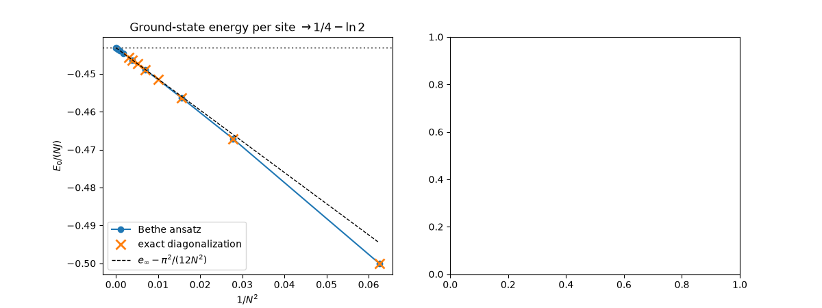
The Bethe equations stay cheap long after exact diagonalization becomes impossible. Conformal field theory predicts \(E_0/N = e_\infty - \pi^2 J / (12 N^2)\) for this \(c = 1\) critical chain.

N_bethe = np.array([4, 6, 8, 12, 16, 24, 32, 48, 64, 128, 256])
e_bethe = np.array([bethe_ansatz_xxx_ground_energy(N) for N in N_bethe]) / N_bethe
e_inf = 0.25 - np.log(2)

fig, axes = plt.subplots(1, 2, figsize=(12, 4.5))
ax = axes[0]
ax.plot(1 / N_bethe**2, e_bethe, "o-", label="Bethe ansatz")
ax.plot(1 / N_ed**2, E_ed / N_ed, "x", ms=10, mew=2, label="exact diagonalization")
x = np.linspace(0, 1 / 16, 50)
ax.plot(x, e_inf - np.pi**2 / 12 * x, "k--", lw=1, label=r"$e_\infty - \pi^2/(12N^2)$")
ax.axhline(e_inf, color="0.5", ls=":")
ax.set_xlabel(r"$1/N^2$")
ax.set_ylabel(r"$E_0 / (NJ)$")
ax.set_title(r"Ground-state energy per site $\to 1/4 - \ln 2$")
ax.legend()

<matplotlib.legend.Legend object at 0x176997da0>

A gapless spectrum

Unlike the integer-spin chain, the spin-1/2 Heisenberg chain has no gap: the singlet-triplet splitting closes as \(1/N\).

ax = axes[1]
ax.plot(1 / N_ed, gap_ed, "o-")
ax.set_xlabel(r"$1/N$")
ax.set_ylabel(r"$E_{S=1} - E_0$ ($J$)")
ax.set_title("Singlet-triplet gap closes linearly in 1/N")
ax.set_xlim(0, None)
ax.set_ylim(0, None)
fig.tight_layout()

Check

Exact diagonalization and the Bethe equations agree to machine precision, and E0/N -> 1/4 - ln 2 with the CFT correction -pi^2 / 12 N^2.

np.testing.assert_allclose(E_ed, E_bethe, atol=1e-8)
assert abs(e_bethe[-1] - (e_inf - np.pi**2 / (12 * N_bethe[-1] ** 2))) < 1e-6
assert np.all(np.diff(gap_ed) < 0)