Calabrese-Cardy: logarithmic entanglement at criticality vs. the area law

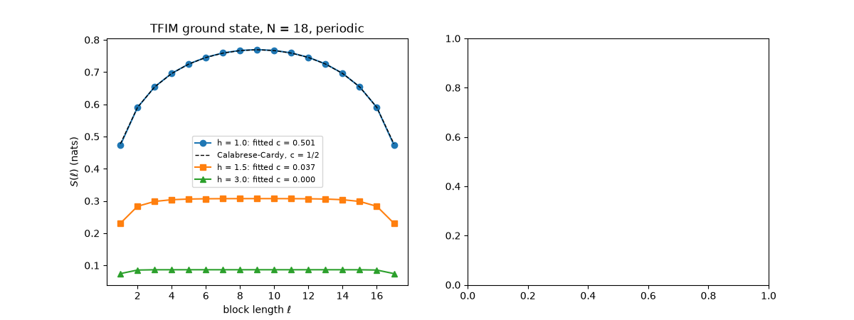
In a gapped chain the entanglement entropy of a block saturates – an “area law”, the boundary of a 1D block being two points. At a quantum critical point Calabrese and Cardy (2004) showed it instead grows as \(S(\ell) = \frac{c}{3}\ln\!\left[\frac{N}{\pi}\sin\frac{\pi\ell}{N}\right] + c'\), with \(c\) the central charge of the conformal field theory. Exact ground states of the transverse-field Ising chain (tfim_hamiltonian()) show both behaviors, and fit_central_charge() recovers the Ising value \(c = 1/2\).

import matplotlib.pyplot as plt
import numpy as np

from physicskit.condensed.spin_chains import (
    calabrese_cardy_entropy,
    entanglement_profile,
    fit_central_charge,
    lowest_eigenstates,
    tfim_hamiltonian,
)


def ground_state_profile(N, h):
    H, basis = tfim_hamiltonian(N, J=1.0, h=h, parity=+1)
    _, V = lowest_eigenstates(H, k=1)
    return entanglement_profile(V[:, 0], N, basis=basis)


N = 18
ell = np.arange(1, N)

Entanglement profile \(S(\ell)\)

fig, axes = plt.subplots(1, 2, figsize=(12, 4.5))
for h, style in ((1.0, "o-"), (1.5, "s-"), (3.0, "^-")):
    S = ground_state_profile(N, h)
    c, const = fit_central_charge(S, N, trim=2)
    axes[0].plot(ell, S, style, label=f"h = {h}: fitted c = {c:.3f}")
    if h == 1.0:
        axes[0].plot(ell, calabrese_cardy_entropy(ell, N, 0.5, const), "k--", lw=1, label="Calabrese-Cardy, c = 1/2")
axes[0].set_xlabel(r"block length $\ell$")
axes[0].set_ylabel(r"$S(\ell)$ (nats)")
axes[0].set_title(f"TFIM ground state, N = {N}, periodic")
axes[0].legend(fontsize=8)

<matplotlib.legend.Legend object at 0x33b782600>

Against the chord length

Plotted against \(\ln[(N/\pi)\sin(\pi\ell/N)]\) the critical profile is a straight line of slope \(c/3\); the gapped one is flat.

for h, style in ((1.0, "o-"), (3.0, "^-")):
    for N_s in (12, 18):
        S = ground_state_profile(N_s, h)
        chord = np.log(N_s / np.pi * np.sin(np.pi * np.arange(1, N_s) / N_s))
        axes[1].plot(chord, S, style, ms=4, label=f"h = {h}, N = {N_s}")
x = np.linspace(0, 1.8, 10)
axes[1].plot(x, x / 6 + fit_central_charge(ground_state_profile(18, 1.0), 18, trim=2)[1], "k--", lw=1, label="slope 1/6")
axes[1].set_xlabel(r"$\ln[(N/\pi)\sin(\pi\ell/N)]$")
axes[1].set_ylabel(r"$S(\ell)$")
axes[1].set_title("Log law at h = J, area law at h = 3J")
axes[1].legend(fontsize=8)
fig.tight_layout()

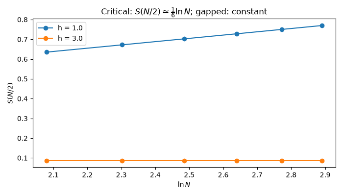
Half-chain entropy vs. system size

sizes = np.arange(8, 19, 2)
fig2, ax2 = plt.subplots(figsize=(7, 4))
for h in (1.0, 3.0):
    S_half = [ground_state_profile(n, h)[n // 2 - 1] for n in sizes]
    ax2.plot(np.log(sizes), S_half, "o-", label=f"h = {h}")
ax2.set_xlabel(r"$\ln N$")
ax2.set_ylabel(r"$S(N/2)$")
ax2.set_title(r"Critical: $S(N/2) \simeq \frac{1}{6}\ln N$; gapped: constant")
ax2.legend()
fig2.tight_layout()

Check

At the critical point the fitted central charge is the Ising value 1/2; deep in the gapped phase the half-chain entropy saturates.

c_crit, _ = fit_central_charge(ground_state_profile(N, 1.0), N, trim=2)
assert abs(c_crit - 0.5) < 0.03
S_gapped = [ground_state_profile(n, 3.0)[n // 2 - 1] for n in (12, 18)]
assert abs(S_gapped[1] - S_gapped[0]) < 1e-3