The transverse-field Ising chain as free fermions

Lieb, Schultz and Mattis (1961) and Pfeuty (1970) mapped the transverse-field Ising chain \(H = -J\sum\sigma^x_i\sigma^x_{i+1} - h\sum\sigma^z_i\) onto free fermions with dispersion \(\varepsilon_k = 2\sqrt{J^2 + h^2 - 2Jh\cos k}\). This example checks the full many-body spectrum from tfim_free_fermion_spectrum() against exact diagonalization of tfim_hamiltonian(), and follows the gap as it closes at the quantum critical point \(h = J\).

import matplotlib.pyplot as plt
import numpy as np

from physicskit.condensed.spin_chains import (
    energy_gap,
    tfim_free_fermion_spectrum,
    tfim_ground_state_energy,
    tfim_hamiltonian,
)

N = 8
h_values = np.linspace(0, 2, 41)

Every one of the \(2^N\) levels is a free-fermion state

fig, axes = plt.subplots(1, 2, figsize=(12, 5))
for parity, color in ((+1, "C0"), (-1, "C3")):
    for h in h_values:
        H, _ = tfim_hamiltonian(N, J=1.0, h=h, parity=parity)
        E_ed = np.linalg.eigvalsh(H.toarray())[:20]
        E_ff = tfim_free_fermion_spectrum(N, 1.0, h, parity=parity)[:20]
        axes[0].plot(np.full_like(E_ed, h), E_ed, "_", color=color, ms=8)
        axes[0].plot(np.full_like(E_ff, h), E_ff, ".", color="k", ms=1.5)
axes[0].plot([], [], "_", color="C0", label=r"ED, parity $P=+1$")
axes[0].plot([], [], "_", color="C3", label=r"ED, parity $P=-1$")
axes[0].plot([], [], ".", color="k", label="free fermions")
axes[0].axvline(1.0, color="0.5", ls=":")
axes[0].set_xlabel("h / J")
axes[0].set_ylabel("E / J")
axes[0].set_title(f"Lowest 20 levels per sector, N = {N}")
axes[0].legend(fontsize=8)

H, _ = tfim_hamiltonian(N, J=1.0, h=0.7)
err = np.abs(tfim_free_fermion_spectrum(N, 1.0, 0.7) - np.linalg.eigvalsh(H.toarray())).max()
print(f"max |ED - free fermion| over all {2**N} levels at h = 0.7: {err:.1e}")

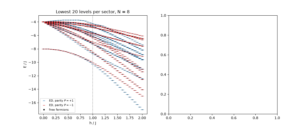
max |ED - free fermion| over all 256 levels at h = 0.7: 3.2e-14

The gap closes at the quantum critical point

The cheapest fermion costs \(\min_k \varepsilon_k = 2|h - J|\). In the ordered phase the two parity sectors become degenerate (the two ferromagnetic states), so we follow the gap within the even sector, where excitations come in pairs: it tends to \(4|h - J|\) on both sides and vanishes only at \(h = J\).

for N_gap in (8, 12, 16):
    gaps = [energy_gap(tfim_hamiltonian(N_gap, J=1.0, h=h, parity=+1)[0]) for h in h_values]
    axes[1].plot(h_values, gaps, label=f"ED even sector, N = {N_gap}")
axes[1].plot(h_values, 4 * np.abs(h_values - 1), "k--", label=r"$4|h - J|$, $N\to\infty$")
axes[1].set_xlabel("h / J")
axes[1].set_ylabel("gap / J")
axes[1].set_title("Gap closing at h = J")
axes[1].legend(fontsize=8)
fig.tight_layout()

Ground-state energy in the thermodynamic limit

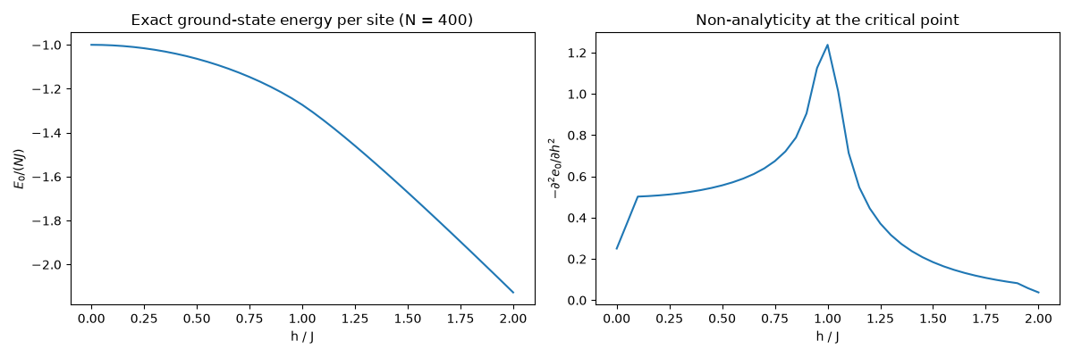
Summing \(-\varepsilon_k/2\) over the Brillouin zone gives the exact ground-state energy, whose second derivative diverges logarithmically at \(h = J\) – the Ising universality class specific-heat singularity.

N_big = 400
e0 = np.array([tfim_ground_state_energy(N_big, 1.0, h) for h in h_values]) / N_big
d2e = np.gradient(np.gradient(e0, h_values), h_values)
fig2, ax2 = plt.subplots(1, 2, figsize=(12, 4))
ax2[0].plot(h_values, e0)
ax2[0].set_xlabel("h / J")
ax2[0].set_ylabel(r"$E_0 / (NJ)$")
ax2[0].set_title(f"Exact ground-state energy per site (N = {N_big})")
ax2[1].plot(h_values, -d2e)
ax2[1].set_xlabel("h / J")
ax2[1].set_ylabel(r"$-\partial^2 e_0/\partial h^2$")
ax2[1].set_title("Non-analyticity at the critical point")
fig2.tight_layout()

Check

Every level is a free-fermion level; the even-sector gap closes only at h = J, and the exact energy per site at h = J is -4/pi.

assert err < 1e-10
gaps16 = np.array([energy_gap(tfim_hamiltonian(16, J=1.0, h=h, parity=+1)[0]) for h in (0.5, 1.0, 1.5)])
assert gaps16[1] < 0.5 * min(gaps16[0], gaps16[2])
assert abs(e0[np.argmin(np.abs(h_values - 1))] + 4 / np.pi) < 1e-4
assert np.argmax(-d2e) == np.argmin(np.abs(h_values - 1))