The 3D Topological Insulator: A Single Surface Dirac Cone

Fu, Kane, and Mele’s 2007 extension of the 2D Z2 classification to three dimensions predicted a bulk insulator whose surface hosts a single, gapless Dirac cone, protected by time-reversal symmetry alone – confirmed directly by ARPES on Bi2Se3 and Bi2Te3 in 2008-2009. topological_insulator_3d_slab_hamiltonian() opens the minimal 4-band lattice model along one direction, exposing exactly this surface state: pinned to zero energy at the surface Brillouin zone center, localized on a single outer layer, and dispersing linearly away from it.

import matplotlib.pyplot as plt
import numpy as np

from physicskit.condensed.topological_insulator_3d import (
    topological_insulator_3d_hamiltonian,
    topological_insulator_3d_slab_hamiltonian,
)

Bulk bands stay gapped; the slab develops a mid-gap surface state

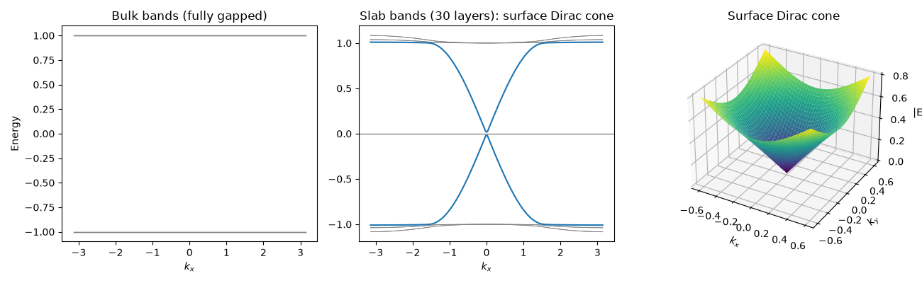
In the strong-topological-insulator window (\(1 < |m/t| < 3\)), the bulk spectrum along any line through the Brillouin zone remains fully gapped, while a slab – open along one direction – develops states pinned inside that gap.

m, t = -2.0, 1.0
n_layers = 30
kx_grid = np.linspace(-np.pi, np.pi, 150)

bulk_bands = np.array([np.linalg.eigvalsh(topological_insulator_3d_hamiltonian(kx, 0.0, 0.0, m=m, t=t)) for kx in kx_grid])
slab_bands = np.array([np.linalg.eigvalsh(topological_insulator_3d_slab_hamiltonian(kx, 0.0, n_layers=n_layers, m=m, t=t)) for kx in kx_grid])

The surface Dirac cone in the (kx, ky) plane

Tracking only the pair of mid-gap slab bands across a 2D grid of (kx, ky) traces out a linear Dirac cone centered at the surface Brillouin zone center – the single cone ARPES resolved directly on Bi2Se3 and Bi2Te3.

k_line = np.linspace(-0.6, 0.6, 41)


def _min_abs_energy(kx, ky):
    eigs = np.linalg.eigvalsh(topological_insulator_3d_slab_hamiltonian(kx, ky, n_layers=n_layers, m=m, t=t))
    return np.min(np.abs(eigs))


cone = np.array([[_min_abs_energy(kx, ky) for ky in k_line] for kx in k_line])

fig = plt.figure(figsize=(13, 4))

ax1 = fig.add_subplot(1, 3, 1)
ax1.plot(kx_grid, bulk_bands, color="gray", lw=1)
ax1.set_xlabel(r"$k_x$")
ax1.set_ylabel("Energy")
ax1.set_title("Bulk bands (fully gapped)")

ax2 = fig.add_subplot(1, 3, 2)
mid = slab_bands.shape[1] // 2
ax2.plot(kx_grid, slab_bands[:, mid - 6 : mid + 6], color="gray", lw=0.6)
ax2.plot(kx_grid, slab_bands[:, mid - 1 : mid + 1], color="C0", lw=1.5)
ax2.axhline(0, color="k", lw=0.5)
ax2.set_xlabel(r"$k_x$")
ax2.set_title(f"Slab bands ({n_layers} layers): surface Dirac cone")

ax3 = fig.add_subplot(1, 3, 3, projection="3d")
KX, KY = np.meshgrid(k_line, k_line, indexing="ij")
ax3.plot_surface(KX, KY, cone, cmap="viridis", linewidth=0, antialiased=True)
ax3.set_xlabel(r"$k_x$")
ax3.set_ylabel(r"$k_y$")
ax3.set_zlabel("|E|")
ax3.set_title("Surface Dirac cone")

fig.tight_layout()

gap_at_gamma = np.min(np.abs(np.linalg.eigvalsh(topological_insulator_3d_slab_hamiltonian(0.0, 0.0, n_layers=n_layers, m=m, t=t))))
print(f"surface-state gap at the Dirac point (Gamma-bar): {gap_at_gamma:.2e}")

surface-state gap at the Dirac point (Gamma-bar): 5.69e-17