The SSH Model: Zak Phase and Protected Edge States

Su, Schrieffer, and Heeger showed that a dimerized chain – alternating intracell hopping \(v\) and intercell hopping \(w\) – is topologically nontrivial whenever \(v < w\): the bulk Zak phase is quantized to \(\pi\), and cutting the chain open exposes a pair of protected, exponentially localized zero-energy states, one at each end. This is the earliest example of the bulk-boundary correspondence. ssh_hamiltonian() gives the closed-form Bloch Hamiltonian, zak_phase() computes the bulk invariant from it, and ssh_lattice_hamiltonian() together with build_finite_cluster() exposes the boundary modes on a finite, open chain – and lets us plot the chain’s actual real-space structure rather than an abstract site-index axis.

import matplotlib.pyplot as plt
import numpy as np

from physicskit.condensed.models import ssh_hamiltonian, ssh_lattice_hamiltonian
from physicskit.condensed.tight_binding import build_finite_cluster
from physicskit.condensed.topology import zak_phase
from physicskit.condensed.visualizers import plot_lattice_structure

The bulk invariant: Zak phase in the two dimerization regimes

The Zak phase is quantized by chiral symmetry to either \(0\) (trivial, \(v>w\)) or \(\pi\) (topological, \(v<w\)) – with nothing in between, since the bulk gap only closes at \(v=w\).

topological = lambda k: ssh_hamiltonian(k, v=0.5, w=1.0)
trivial = lambda k: ssh_hamiltonian(k, v=1.0, w=0.5)

zak_topological = zak_phase(topological)
zak_trivial = zak_phase(trivial)
print(f"Zak phase, v<w (topological): {zak_topological:.4f}  (expect +-pi)")
print(f"Zak phase, v>w (trivial):     {zak_trivial:.4f}  (expect 0)")

Zak phase, v<w (topological): -3.1416  (expect +-pi)
Zak phase, v>w (trivial):     -0.0000  (expect 0)

Bulk-boundary correspondence: the finite chain’s real-space structure

The Zak phase is a purely bulk (periodic-boundary) quantity. Cutting the topological chain (\(v<w\)) into a finite, open wire produces a pair of near-degenerate mid-gap states pinned to zero energy – exactly the correspondence the Zak phase predicts. Because the two are numerically degenerate, numpy.linalg.eigh() returns an arbitrary basis of that two-dimensional subspace rather than the individual left- and right-localized modes; summing both states’ densities recovers the physical picture, exponentially localized at both ends and vanishing on every other (B-sublattice) site.

Drawing the chain’s real structure – rather than density against a bare site index – also makes the mechanism visible directly: bond linewidth below is drawn proportional to hopping strength, so the weak \(v\) bond exposed at each open end is exactly what leaves those end sites undercoordinated and hosting the protected zero mode.

v, w, n_cells = 0.5, 1.0, 15
H, positions, bonds = build_finite_cluster(ssh_lattice_hamiltonian(v=v, w=w), n_cells=n_cells)

spectrum, states = np.linalg.eigh(H)
edge_idx = np.argsort(np.abs(spectrum))[:2]
density = np.abs(states[:, edge_idx[0]]) ** 2 + np.abs(states[:, edge_idx[1]]) ** 2

fig, (ax1, ax2) = plt.subplots(1, 2, figsize=(11, 4.5))

ax1.bar(["trivial (v>w)", "topological (v<w)"], [abs(zak_trivial), abs(zak_topological)], color=["C0", "C1"])
ax1.axhline(np.pi, color="gray", ls="--", label=r"$\pi$")
ax1.set_ylabel("|Zak phase|")
ax1.set_title("Bulk invariant")
ax1.legend()

plot_lattice_structure(positions, bonds, weights=density, ax=ax2)
ax2.set_title(f"Zero-mode density, |E| = {abs(spectrum[edge_idx[0]]):.2e}")
ax2.set_ylim(-0.5, 0.5)

fig.suptitle("SSH model: Zak phase pi <=> protected zero-energy edge states")
fig.tight_layout()

left_weight, right_weight = density[: len(density) // 2].sum(), density[len(density) // 2 :].sum()
print(f"zero-mode weight -- left half: {left_weight:.3f}, right half: {right_weight:.3f}")

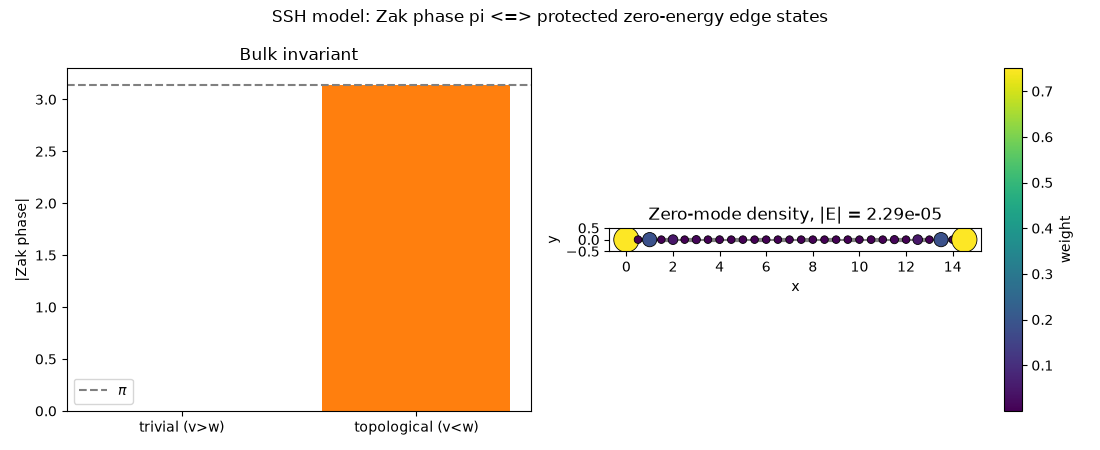
zero-mode weight -- left half: 1.000, right half: 1.000