Quantum Spin Hall Effect: Konig et al.’s Helical Edge States

Konig, Molenkamp, and coworkers measured a quantized two-terminal conductance of \(2e^2/h\) in HgTe/CdTe quantum wells in 2007 – the first experimentally realized topological insulator, and the direct confirmation of the band-inverted BHZ model. Opening the BHZ ribbon along one direction with bhz_ribbon_hamiltonian() exposes exactly the pair of helical, counter-propagating edge states carrying that dissipationless conductance: gapless at \(k_x=0\), spin-locked, and immune to backscattering by nonmagnetic disorder.

import matplotlib.pyplot as plt
import numpy as np

from physicskit.condensed.models import bhz_hamiltonian, bhz_ribbon_hamiltonian
from physicskit.condensed.topology import z2_invariant

Ribbon band structure: topological vs trivial band inversion

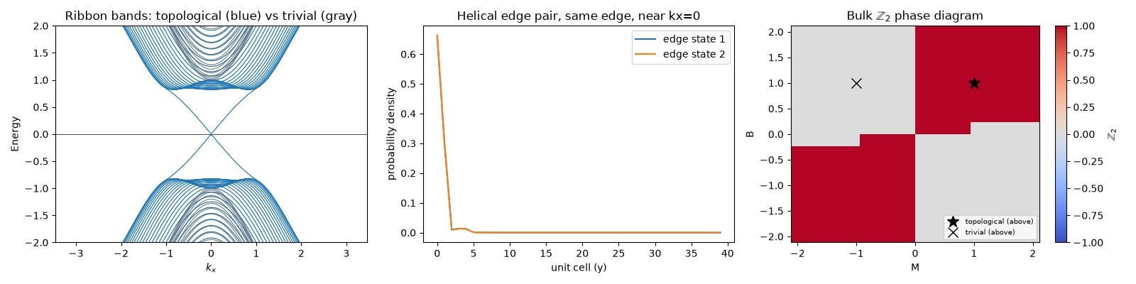
In the band-inverted regime (M/B > 0) a pair of edge bands crosses inside the bulk gap at k_x=0; in the uninverted regime (M/B < 0) the ribbon is a simple gapped insulator with no such crossing.

n_cells = 40
kx_grid = np.linspace(-np.pi, np.pi, 200)

bands_topological = np.array([np.linalg.eigvalsh(bhz_ribbon_hamiltonian(kx, n_cells, M=1.0, B=1.0)) for kx in kx_grid])
bands_trivial = np.array([np.linalg.eigvalsh(bhz_ribbon_hamiltonian(kx, n_cells, M=-1.0, B=1.0)) for kx in kx_grid])

Real-space profile of the near-zero edge modes

Exactly at k_x=0 the edge states are degenerate and any linear combination is a valid eigenvector, so a diagonalizer may return them already mixed. A hair away from the crossing lifts that ambiguity: the two spin-locked, counter-propagating branches on the same edge – the helical pair – localize cleanly.

H_k = bhz_ribbon_hamiltonian(kx=0.1, n_cells=n_cells, M=1.0, B=1.0)
eigs, vecs = np.linalg.eigh(H_k)
mid = len(eigs) // 2
edge_state_1 = vecs[:, mid - 1]
edge_state_2 = vecs[:, mid]
density_1 = np.sum(np.abs(edge_state_1.reshape(n_cells, 4)) ** 2, axis=1)
density_2 = np.sum(np.abs(edge_state_2.reshape(n_cells, 4)) ** 2, axis=1)
print(f"near-zero energies at kx=0.1: {eigs[mid - 1]:.4f}, {eigs[mid]:.4f}")
print(f"edge state 1 (E={eigs[mid - 1]:.3f}) weight on first/last 3 cells: {density_1[:3].sum():.4f} / {density_1[-3:].sum():.4f}")
print(f"edge state 2 (E={eigs[mid]:.3f}) weight on first/last 3 cells: {density_2[:3].sum():.4f} / {density_2[-3:].sum():.4f}")

near-zero energies at kx=0.1: -0.0998, 0.0998
edge state 1 (E=-0.100) weight on first/last 3 cells: 0.9720 / 0.0000
edge state 2 (E=0.100) weight on first/last 3 cells: 0.9720 / 0.0000

Where do M=1 and M=-1 sit on the full bulk phase diagram?

The two ribbon calculations above are two points on a much larger picture: gridding the bulk z2_invariant() over both M and B traces the whole band-inversion phase boundary at once, showing exactly why M/B > 0 (band-inverted) is the condition for the edge states seen above.

M_grid = np.linspace(-2.0, 2.0, 18)
B_grid = np.linspace(-2.0, 2.0, 18)
z2_phase = np.array(
    [[z2_invariant(lambda k1, k2, M=M, B=B: bhz_hamiltonian(k1, k2, M=M, B=B), grid_size=14) for M in M_grid] for B in B_grid],
)

fig, axes = plt.subplots(1, 3, figsize=(16, 4))

n_show = 8
axes[0].plot(kx_grid, bands_trivial[:, n_show : 4 * n_cells - n_show], color="gray", lw=0.6)
axes[0].plot(kx_grid, bands_topological[:, n_show : 4 * n_cells - n_show], color="C0", lw=0.6)
axes[0].axhline(0, color="k", lw=0.5)
axes[0].set_xlabel(r"$k_x$")
axes[0].set_ylabel("Energy")
axes[0].set_title("Ribbon bands: topological (blue) vs trivial (gray)")
axes[0].set_ylim(-2, 2)

axes[1].plot(density_1, label="edge state 1")
axes[1].plot(density_2, label="edge state 2")
axes[1].set_xlabel("unit cell (y)")
axes[1].set_ylabel("probability density")
axes[1].set_title("Helical edge pair, same edge, near kx=0")
axes[1].legend()

im = axes[2].pcolormesh(M_grid, B_grid, z2_phase, cmap="coolwarm", shading="auto", vmin=-1, vmax=1)
axes[2].plot([1.0], [1.0], "k*", ms=12, label="topological (above)")
axes[2].plot([-1.0], [1.0], "kx", ms=10, label="trivial (above)")
axes[2].set_xlabel("M")
axes[2].set_ylabel("B")
axes[2].set_title(r"Bulk $\mathbb{Z}_2$ phase diagram")
axes[2].legend(fontsize=7, loc="lower right")
fig.colorbar(im, ax=axes[2], label=r"$\mathbb{Z}_2$")

fig.tight_layout()