The Kitaev Chain: Unpaired Majorana Zero Modes

Alexei Kitaev showed that a 1D spinless p-wave superconductor hosts unpaired Majorana zero modes – particles that are their own antiparticles – localized at the two ends of an open chain, whenever the chemical potential satisfies \(|\mu| < 2t\). A pair of spatially separated Majoranas encodes one nonlocal fermionic degree of freedom immune to local perturbations, making the Kitaev chain the founding proposal for topologically protected quantum computation. kitaev_chain_hamiltonian() gives the bulk (periodic) BdG Bloch Hamiltonian used to confirm the bulk gap stays open, and kitaev_chain_bdg_real_space() builds the open chain that exposes the Majorana end modes directly in the spectrum – plotted below as a real-space structure so the two end modes are visible directly on the chain rather than as an abstract site index.

import matplotlib.pyplot as plt
import numpy as np

from physicskit.condensed.models import kitaev_chain_bdg_real_space, kitaev_chain_hamiltonian
from physicskit.condensed.visualizers import plot_lattice_structure

The bulk BdG spectrum stays gapped in the topological regime

With periodic boundary conditions the chain has a fully gapped quasiparticle spectrum – the topology lives entirely in how that bulk gap connects to the boundary, not in the bulk spectrum itself.

mu, t, delta = 0.0, 1.0, 1.0
k_grid = np.linspace(0, 2 * np.pi, 300)
bulk_bands = np.array([np.linalg.eigvalsh(kitaev_chain_hamiltonian(k, mu=mu, t=t, delta=delta)) for k in k_grid])
print(f"bulk gap (min |E| over k): {np.min(np.abs(bulk_bands)):.4f}  (|mu|={abs(mu)} < 2t={2 * t}: topological)")

bulk gap (min |E| over k): 2.0000  (|mu|=0.0 < 2t=2.0: topological)

Cutting the chain open exposes unpaired Majorana end modes

In the real-space, open-boundary BdG Hamiltonian, the bulk gap survives in the interior, but a pair of near-zero-energy states appears – exactly degenerate to machine precision. Because they are degenerate, eigh returns an arbitrary basis of that two-dimensional subspace rather than the two spatially separated Majoranas individually; each basis vector it happens to return is still fully localized at one end or the other, and the two together account for the whole subspace.

N = 60
H_open = kitaev_chain_bdg_real_space(n_sites=N, mu=mu, t=t, delta=delta)
energies, states = np.linalg.eigh(H_open)
zero_idx = np.argsort(np.abs(energies))[:2]
psi_a, psi_b = states[:, zero_idx[0]], states[:, zero_idx[1]]

density_a = np.abs(psi_a[:N]) ** 2 + np.abs(psi_a[N:]) ** 2
density_b = np.abs(psi_b[:N]) ** 2 + np.abs(psi_b[N:]) ** 2

positions = np.column_stack([np.arange(N), np.zeros(N)])
bonds = [(i, i + 1, t) for i in range(N - 1)]

fig, (ax1, ax2) = plt.subplots(1, 2, figsize=(11, 4.5))

ax1.plot(k_grid, bulk_bands, color="C0")
ax1.set_xlabel("k")
ax1.set_ylabel("Energy")
ax1.set_title("Bulk BdG spectrum (periodic chain, fully gapped)")

plot_lattice_structure(positions, bonds, weights=density_a + density_b, ax=ax2)
ax2.set_ylim(-0.5, 0.5)
ax2.set_title(f"Combined Majorana weight, |E| ~ {abs(energies[zero_idx[0]]):.1e}")

fig.suptitle("Kitaev chain: gapped bulk, unpaired Majorana modes at open ends")
fig.tight_layout()

left_a, right_a = density_a[: N // 4].sum(), density_a[-N // 4 :].sum()
left_b, right_b = density_b[: N // 4].sum(), density_b[-N // 4 :].sum()
print(f"mode a weight -- left quarter: {left_a:.3f}, right quarter: {right_a:.3f}")
print(f"mode b weight -- left quarter: {left_b:.3f}, right quarter: {right_b:.3f}")

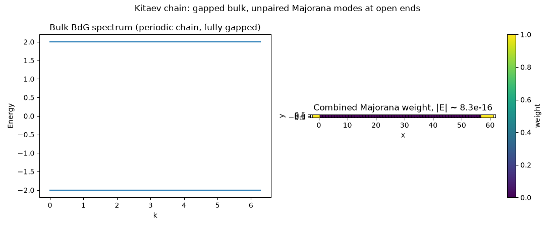
mode a weight -- left quarter: 1.000, right quarter: 0.000
mode b weight -- left quarter: 0.000, right quarter: 1.000