Kane-Mele: Helical Edge States from Two Time-Reversed Haldane Copies

Kane-Mele and BHZ: Z2 Topological Insulators computes the bulk \(\mathbb{Z}_2\) invariant of the Kane-Mele model directly from its Bloch Hamiltonian. This example instead looks at what that invariant predicts on a finite sample. Whenever the Rashba term vanishes, \(s_z\) is conserved and kane_mele_hamiltonian() is exactly block-diagonal in spin – two independent Haldane models with opposite next-nearest-neighbor phase, \(\phi\) and \(-\phi\). Building each spin’s finite flake separately with build_finite_cluster() (the same disk-shaped cut used in The Haldane Model: a Chiral Edge State on an Arbitrary Boundary) shows both spins independently host a boundary-hugging state at the same real-space locations – a Kramers pair – while a momentum-resolved ribbon dispersion shows the two spins cross the gap with opposite group velocity, the helical counter-propagation that makes the quantum spin Hall edge robust against time-reversal-preserving disorder.

import matplotlib.pyplot as plt
import numpy as np

from physicskit.condensed.models import haldane_lattice_hamiltonian
from physicskit.condensed.tight_binding import Lattice, build_finite_cluster, build_ribbon
from physicskit.condensed.visualizers import plot_lattice_structure

t, lambda_so = 1.0, 0.2

Helical dispersion: opposite group velocity for opposite spin

Each spin sees a Haldane ribbon with \(t_2 = \lambda_{so}\) and \(\phi = \pm\pi/2\). Both host a chiral edge band crossing the bulk gap, but with opposite sign of \(\phi\) the two crossings run in opposite directions – spin-up and spin-down edge modes counter-propagate at the same boundary.

n_ribbon = 20
k_grid = np.linspace(-np.pi, np.pi, 300)
H_ribbon_up = build_ribbon(haldane_lattice_hamiltonian(t=t, t2=lambda_so, phi=np.pi / 2, M=0.0), open_direction=0, n_cells=n_ribbon)
H_ribbon_dn = build_ribbon(haldane_lattice_hamiltonian(t=t, t2=lambda_so, phi=-np.pi / 2, M=0.0), open_direction=0, n_cells=n_ribbon)
bands_up = np.array([np.linalg.eigvalsh(H_ribbon_up(k)) for k in k_grid])
bands_dn = np.array([np.linalg.eigvalsh(H_ribbon_dn(k)) for k in k_grid])

Real-space Kramers pair: both spins hug the same disordered boundary

Cutting a disk out of the lattice – an edge with no crystallographic meaning – still traps both spin species at the boundary, and, because they are exact time-reversal partners, at identical real-space density.

n_cells, radius = 14, 6.0
lat = Lattice.honeycomb()
center = np.array([n_cells / 2, n_cells / 2]) @ lat.lattice_vectors


def in_disk(cell, orbital, position):
    return np.linalg.norm(position - center) <= radius


H_up, positions, bonds = build_finite_cluster(haldane_lattice_hamiltonian(t=t, t2=lambda_so, phi=np.pi / 2, M=0.0), n_cells=(n_cells, n_cells), keep=in_disk)
H_dn, positions_dn, _ = build_finite_cluster(haldane_lattice_hamiltonian(t=t, t2=lambda_so, phi=-np.pi / 2, M=0.0), n_cells=(n_cells, n_cells), keep=in_disk)
assert np.allclose(positions, positions_dn)

eigenvalues_up, eigenvectors_up = np.linalg.eigh(H_up)
eigenvalues_dn, eigenvectors_dn = np.linalg.eigh(H_dn)
mid = len(eigenvalues_up) // 2
gap = slice(mid - 3, mid + 3)
density_up = np.sum(np.abs(eigenvectors_up[:, gap]) ** 2, axis=1)
density_dn = np.sum(np.abs(eigenvectors_dn[:, gap]) ** 2, axis=1)
print(f"max |density_up - density_down| over all sites: {np.max(np.abs(density_up - density_dn)):.2e}  (Kramers partners coincide)")

r = np.linalg.norm(positions - center, axis=1)
weighted_radius = np.sum(r * density_up) / density_up.sum()
print(f"mean site radius: {r.mean():.2f}, density-weighted radius of near-gap states: {weighted_radius:.2f}  (disk radius = {radius:.1f})")

fig, (ax1, ax2) = plt.subplots(1, 2, figsize=(11, 5))

ax1.plot(k_grid, bands_up, color="C0", lw=0.8)
ax1.plot([], [], color="C0", label=r"spin up ($\phi=+\pi/2$)")
ax1.plot(k_grid, bands_dn, color="C1", lw=0.8, ls="--")
ax1.plot([], [], color="C1", ls="--", label=r"spin down ($\phi=-\pi/2$)")
ax1.set_xlabel(r"$k_\parallel$")
ax1.set_ylabel("Energy")
ax1.set_title("Ribbon spectrum: counter-propagating edge bands")
ax1.legend(fontsize=8)

plot_lattice_structure(positions, bonds, weights=density_up, ax=ax2)
ax2.set_title("Spin-up (= spin-down) near-gap density")

fig.suptitle("Kane-Mele model: a Kramers pair of helical edge states")
fig.tight_layout()

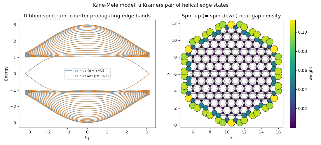
max |density_up - density_down| over all sites: 0.00e+00  (Kramers partners coincide)
mean site radius: 3.98, density-weighted radius of near-gap states: 5.55  (disk radius = 6.0)