Kane-Mele and BHZ: Z2 Topological Insulators

Kane and Mele showed that adding intrinsic spin-orbit coupling to graphene – two time-reversed copies of Haldane’s model, one per spin – produces a time-reversal-symmetric insulator with a new, \(\mathbb{Z}_2\)-valued topological invariant protecting helical, counter-propagating edge states: the quantum spin Hall effect. Bernevig, Hughes, and Zhang then predicted the same physics in HgTe/CdTe quantum wells (the BHZ model), later observed experimentally – the first realized topological insulator. kane_mele_hamiltonian() and bhz_hamiltonian() provide both microscopic realizations, and z2_invariant() extracts the \(\mathbb{Z}_2\) invariant from each via the spin-Chern-number reduction valid whenever \(s_z\) is conserved.

import matplotlib.pyplot as plt
import numpy as np

from physicskit.condensed.models import bhz_hamiltonian, kane_mele_hamiltonian
from physicskit.condensed.topology import compute_chern_number, z2_invariant

Kane-Mele: turning on spin-orbit coupling drives a Z2 transition

With lambda_so=0 the two spin sectors are decoupled trivial bands; turning on intrinsic spin-orbit coupling makes each spin sector a Haldane Chern insulator with opposite Chern number, so the total Chern number stays zero (time-reversal symmetric) while the Z2 invariant – the spin-up Chern number mod 2 – flips from trivial to topological.

kane_mele_trivial = lambda k1, k2: kane_mele_hamiltonian(k1, k2, lambda_so=0.0)
kane_mele_topological = lambda k1, k2: kane_mele_hamiltonian(k1, k2, lambda_so=0.06)

z2_km_trivial = z2_invariant(kane_mele_trivial, grid_size=20)
z2_km_topological = z2_invariant(kane_mele_topological, grid_size=20)
print(f"Kane-Mele Z2, lambda_so=0.00: {z2_km_trivial}  (trivial)")
print(f"Kane-Mele Z2, lambda_so=0.06: {z2_km_topological}  (quantum spin Hall)")

Kane-Mele Z2, lambda_so=0.00: 0  (trivial)
Kane-Mele Z2, lambda_so=0.06: 1  (quantum spin Hall)

BHZ: band inversion drives the same transition in a 4-band model

The BHZ model’s spin-up block is a 2x2 Dirac Hamiltonian; its Chern number (computed on the isolated spin-up block, as z2_invariant() does internally) is nonzero only when the band- inversion mass \(M\) and curvature \(B\) have the same sign.

bhz_trivial = lambda k1, k2: bhz_hamiltonian(k1, k2, M=-1.0, B=1.0)
bhz_topological = lambda k1, k2: bhz_hamiltonian(k1, k2, M=1.0, B=1.0)

z2_bhz_trivial = z2_invariant(bhz_trivial, grid_size=20)
z2_bhz_topological = z2_invariant(bhz_topological, grid_size=20)
print(f"BHZ Z2, M/B=-1 (no inversion): {z2_bhz_trivial}  (trivial)")
print(f"BHZ Z2, M/B=+1 (inverted):     {z2_bhz_topological}  (topological)")

BHZ Z2, M/B=-1 (no inversion): 0  (trivial)
BHZ Z2, M/B=+1 (inverted):     1  (topological)

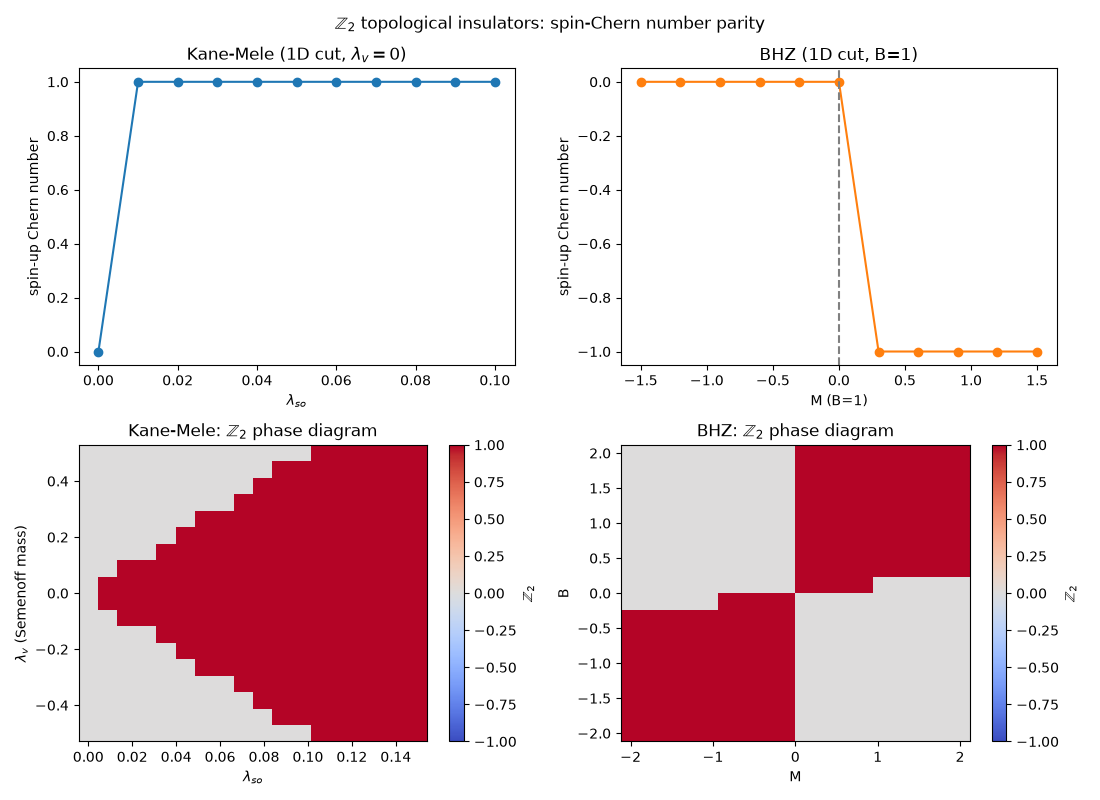
The underlying spin-up Chern numbers behind each Z2 value

Plotting the spin-up-sector Chern number for both models across their respective tuning parameters shows the same story: an odd spin-Chern number gives \(\mathbb{Z}_2=1\), an even one gives \(0\).

lambda_so_values = np.linspace(0.0, 0.1, 11)


def spin_up_chern(hf):
    return compute_chern_number(lambda k1, k2: np.asarray(hf(k1, k2), dtype=complex)[:2, :2], grid_size=20)[0]


km_chern = [spin_up_chern(lambda k1, k2, ls=ls: kane_mele_hamiltonian(k1, k2, lambda_so=ls)) for ls in lambda_so_values]

M_values = np.linspace(-1.5, 1.5, 11)
bhz_chern = [spin_up_chern(lambda k1, k2, M=M: bhz_hamiltonian(k1, k2, M=M, B=1.0)) for M in M_values]

Full 2D phase diagrams: both tuning parameters at once

The 1D cuts above each fix one parameter (a sublattice mass for Kane-Mele, the curvature B for BHZ) and scan the other. Both models actually have two independent tuning knobs – Kane-Mele’s spin-orbit coupling \(\lambda_{so}\) against its sublattice (Semenoff) mass \(\lambda_v\), and BHZ’s inversion mass \(M\) against its curvature \(B\) – so the full phase boundary is a curve in a 2D parameter plane, not a single crossing point on a line. Gridding z2_invariant() over both parameters at once traces that whole boundary directly.

lambda_so_grid = np.linspace(0.0, 0.15, 18)
lambda_v_grid = np.linspace(-0.5, 0.5, 18)


def _km_z2(ls: float, lv: float) -> int:
    return z2_invariant(lambda k1, k2: kane_mele_hamiltonian(k1, k2, lambda_so=ls, lambda_v=lv), grid_size=14)


km_phase = np.array([[_km_z2(ls, lv) for ls in lambda_so_grid] for lv in lambda_v_grid])

M_grid = np.linspace(-2.0, 2.0, 18)
B_grid = np.linspace(-2.0, 2.0, 18)
bhz_phase = np.array(
    [[z2_invariant(lambda k1, k2, M=M, B=B: bhz_hamiltonian(k1, k2, M=M, B=B), grid_size=14) for M in M_grid] for B in B_grid],
)

fig, axd = plt.subplot_mosaic([["km_line", "bhz_line"], ["km_phase", "bhz_phase"]], figsize=(11, 8))

axd["km_line"].plot(lambda_so_values, km_chern, "o-")
axd["km_line"].set_xlabel(r"$\lambda_{so}$")
axd["km_line"].set_ylabel("spin-up Chern number")
axd["km_line"].set_title("Kane-Mele (1D cut, $\\lambda_v=0$)")

axd["bhz_line"].plot(M_values, bhz_chern, "o-", color="C1")
axd["bhz_line"].axvline(0, color="gray", ls="--")
axd["bhz_line"].set_xlabel("M (B=1)")
axd["bhz_line"].set_ylabel("spin-up Chern number")
axd["bhz_line"].set_title("BHZ (1D cut, B=1)")

im1 = axd["km_phase"].pcolormesh(lambda_so_grid, lambda_v_grid, km_phase, cmap="coolwarm", shading="auto", vmin=-1, vmax=1)
axd["km_phase"].set_xlabel(r"$\lambda_{so}$")
axd["km_phase"].set_ylabel(r"$\lambda_v$ (Semenoff mass)")
axd["km_phase"].set_title(r"Kane-Mele: $\mathbb{Z}_2$ phase diagram")
fig.colorbar(im1, ax=axd["km_phase"], label=r"$\mathbb{Z}_2$")

im2 = axd["bhz_phase"].pcolormesh(M_grid, B_grid, bhz_phase, cmap="coolwarm", shading="auto", vmin=-1, vmax=1)
axd["bhz_phase"].set_xlabel("M")
axd["bhz_phase"].set_ylabel("B")
axd["bhz_phase"].set_title(r"BHZ: $\mathbb{Z}_2$ phase diagram")
fig.colorbar(im2, ax=axd["bhz_phase"], label=r"$\mathbb{Z}_2$")

fig.suptitle(r"$\mathbb{Z}_2$ topological insulators: spin-Chern number parity")
fig.tight_layout()