The Integer Quantum Hall Effect: Quantized Hall Conductance from Chern Numbers

Von Klitzing, Dorda, and Pepper’s 1980 discovery – a two-dimensional electron gas in a strong magnetic field develops a Hall conductance quantized to extraordinary precision, \(\sigma_{xy} = \nu\,e^2/h\) with \(\nu\) an exact integer – is reproduced here on its lattice (Bloch) incarnation, the Harper-Hofstadter model (harper_hofstadter_hamiltonian()): a square lattice threaded by a uniform flux \(p/q\) per plaquette. At flux \(1/3\) the spectrum splits into three magnetic sub-bands; feeding each one, in turn, into compute_chern_number() (the same TKNN machinery used for the Haldane model) gives the exact integer Chern number of that band, and summing the Chern numbers of every filled band below a gap gives that gap’s quantized Hall conductance directly – the numerical content of the TKNN formula that explains why von Klitzing’s measurement came out an integer at all.

import matplotlib.pyplot as plt
import numpy as np

from physicskit.condensed.models import harper_hofstadter_hamiltonian
from physicskit.condensed.topology import compute_chern_number

Three magnetic sub-bands at flux 1/3

Odd q avoids the exact band touchings that occur for some even flux denominators, where individual-band Chern numbers become ill-defined.

p, q = 1, 3
k2_grid = np.linspace(0, 2 * np.pi, 200)
bands = np.array([np.linalg.eigvalsh(harper_hofstadter_hamiltonian(0.0, k2, p, q)) for k2 in k2_grid])

chern_numbers = compute_chern_number(lambda k1, k2: harper_hofstadter_hamiltonian(k1, k2, p, q), grid_size=30)
sigma_xy = np.cumsum(chern_numbers)
print(f"flux = {p}/{q}: band Chern numbers = {chern_numbers} (sum = {sum(chern_numbers)})")
print(f"quantized Hall conductance below each gap (units of e^2/h): {list(sigma_xy[:-1])}")

fig, (ax1, ax2) = plt.subplots(1, 2, figsize=(11, 4.3))
for n in range(q):
    ax1.plot(k2_grid, bands[:, n], color="steelblue")
ax1.set_xlabel(r"$k_2$")
ax1.set_ylabel("E")
ax1.set_title(f"Hofstadter sub-bands at flux {p}/{q} (k1 = 0)")

ax2.bar(range(1, q + 1), sigma_xy, color="firebrick")
ax2.axhline(0, color="black", lw=0.5)
ax2.set_xticks(range(1, q + 1))
ax2.set_xlabel("bands filled")
ax2.set_ylabel(r"$\sigma_{xy}$  ($e^2/h$)")
ax2.set_title("Quantized Hall conductance below each gap")
fig.tight_layout()

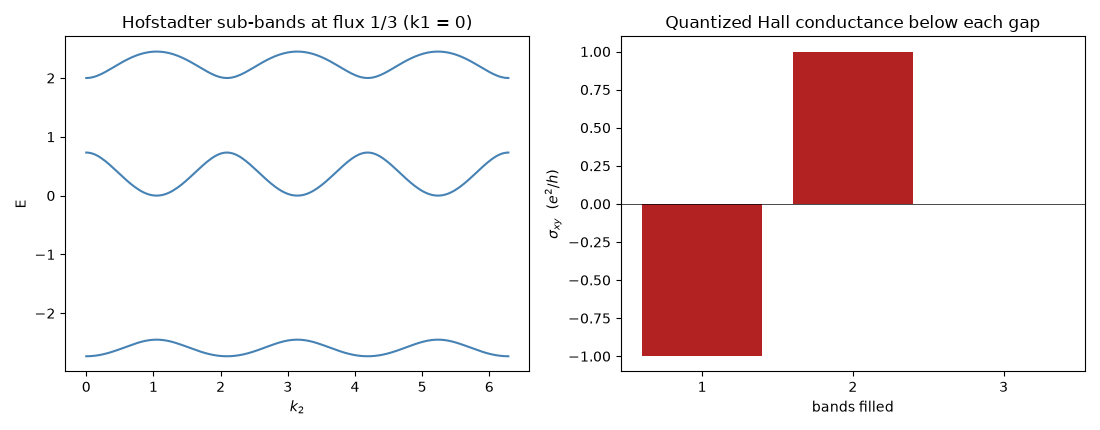
flux = 1/3: band Chern numbers = [-1, 2, -1] (sum = 0)
quantized Hall conductance below each gap (units of e^2/h): [np.int64(-1), np.int64(1)]

Every gap’s conductance is an exact integer, and the three bands’ Chern numbers sum to exactly zero – the full three-band Hilbert space, taken together, is topologically trivial, as it must be for any complete set of bands of a lattice Hamiltonian; the nontrivial physics is entirely in how that zero splits across the individual gaps.

plt.show()