The Drude model: conductivity and the Hall effect

Three years after the discovery of the electron, Paul Drude (1900) treated the electrons of a metal as a classical gas, accelerated by fields and randomized by collisions every \(\tau\) on average. This gives Ohm’s law with \(\sigma_0 = nq^2\tau/m\) (drude_conductivity()), a Lorentzian AC response (drude_ac_conductivity()), and, in a magnetic field, a Hall resistivity \(\rho_{yx} = B/(nq)\) with no magnetoresistance (drude_conductivity_tensor()).

import matplotlib.pyplot as plt
import numpy as np

from physicskit.condensed.transport import (
    drude_ac_conductivity,
    drude_conductivity,
    drude_conductivity_tensor,
    hall_coefficient,
)

n, tau, q, m = 1.0, 1.0, -1.0, 1.0
sigma0 = drude_conductivity(n, tau, q, m)

Optical conductivity

The real part is a Lorentzian of width \(1/\tau\) (the “Drude peak” of metals’ infrared absorption); its area is fixed by the f-sum rule, \(\int_0^\infty \mathrm{Re}\,\sigma\,d\omega = \pi nq^2/2m\), whatever \(\tau\) is.

omega = np.linspace(0, 6, 400)
fig, axes = plt.subplots(1, 2, figsize=(12, 4.5))
for t in (0.5, 1.0, 3.0):
    s = drude_ac_conductivity(omega, n, t, q, m)
    axes[0].plot(omega, s.real, lw=2, label=rf"Re $\sigma$, $\tau = {t}$")
    area = np.trapezoid(drude_ac_conductivity(np.linspace(0, 2000, 400001), n, t, q, m).real, dx=2000 / 400000)
    print(f"tau = {t}: sum-rule integral = {area:.4f} (pi n q^2 / 2m = {np.pi / 2:.4f})")
s1 = drude_ac_conductivity(omega, n, 1.0, q, m)
axes[0].plot(omega, s1.imag, "k--", lw=1, label=r"Im $\sigma$, $\tau = 1$")
axes[0].set_xlabel(r"$\omega$")
axes[0].set_ylabel(r"$\sigma(\omega)$")
axes[0].set_title("Drude AC conductivity")
axes[0].legend(fontsize=8)

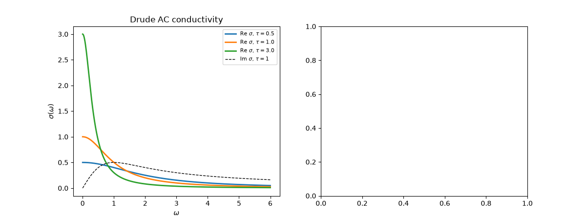
tau = 0.5: sum-rule integral = 1.5698 (pi n q^2 / 2m = 1.5708)
tau = 1.0: sum-rule integral = 1.5703 (pi n q^2 / 2m = 1.5708)
tau = 3.0: sum-rule integral = 1.5706 (pi n q^2 / 2m = 1.5708)

<matplotlib.legend.Legend object at 0x3706ca390>

Hall effect and magnetoresistance

In a field \(B\hat z\) the Lorentz force deflects the current until a transverse Hall field builds up. \(\rho_{yx}\) grows linearly in \(B\) with slope \(R_H = 1/(nq)\), whose sign gives the sign of the carriers’ charge, while \(\rho_{xx}\) stays at \(1/\sigma_0\).

B = np.linspace(-5, 5, 101)
for charge, style in ((-1.0, "-"), (+1.0, "--")):
    rho = np.array([np.linalg.inv(drude_conductivity_tensor(b, n, tau, charge, m)) for b in B])
    axes[1].plot(B, rho[:, 1, 0], style, lw=2, label=rf"$\rho_{{yx}}$, q = {charge:+.0f}")
    axes[1].plot(B, rho[:, 0, 0], style, color="0.5", lw=1, label=rf"$\rho_{{xx}}$, q = {charge:+.0f}")
axes[1].set_xlabel("B")
axes[1].set_ylabel(r"resistivity")
axes[1].set_title(rf"Hall resistivity: slope $R_H = 1/nq = {hall_coefficient(n, q):+.0f}$")
axes[1].legend(fontsize=8)
fig.tight_layout()

Current in crossed fields

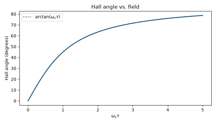
With \(\mathbf E = E\hat x\), the Hall angle \(\tan\theta_H = \omega_c\tau\) rotates the current away from the field direction.

wct = np.linspace(0, 5, 100)
sigma_xx = np.array([drude_conductivity_tensor(w / tau, n, tau, -q, m)[0, 0] for w in wct])
sigma_yx = np.array([drude_conductivity_tensor(w / tau, n, tau, -q, m)[1, 0] for w in wct])
fig2, ax2 = plt.subplots(figsize=(7, 4))
ax2.plot(wct, np.degrees(np.arctan2(-sigma_yx, sigma_xx)), lw=2)
ax2.plot(wct, np.degrees(np.arctan(wct)), "k:", label=r"$\arctan(\omega_c\tau)$")
ax2.set_xlabel(r"$\omega_c\tau$")
ax2.set_ylabel("Hall angle (degrees)")
ax2.set_title("Hall angle vs. field")
ax2.legend()
fig2.tight_layout()

Check

f-sum rule; rho_xx = 1/sigma_0 independent of B (no magnetoresistance); R_H = 1/(nq); Hall angle arctan(omega_c tau).

assert abs(area - np.pi / 2) < 1e-3
np.testing.assert_allclose(rho[:, 0, 0], 1 / sigma0, rtol=1e-12)
np.testing.assert_allclose(np.abs(rho[:, 1, 0]), np.abs(B) / n, rtol=1e-12, atol=1e-12)
assert np.isclose(hall_coefficient(n, q), 1 / (n * q))
np.testing.assert_allclose(np.arctan2(-sigma_yx, sigma_xx), np.arctan(wct), atol=1e-12)