Sommerfeld’s electron gas: the Wiedemann-Franz law and thermopower

Drude’s classical gas got the conductivity right but the electronic heat capacity and thermopower wrong by factors of order \(k_BT/E_F\). Sommerfeld (1927-1928) kept the kinetic picture but used Fermi-Dirac statistics. Only electrons within \(k_BT\) of the Fermi energy carry current or heat. The Boltzmann equation in the relaxation-time approximation (boltzmann_transport()) then gives, for any band, the Wiedemann-Franz law \(\kappa/\sigma T = \pi^2/3\) (\(k_B = e = 1\)) and Mott’s formula for the Seebeck coefficient. This example checks both on a 2D tight-binding band sampled on a \(k\)-grid.

import matplotlib.pyplot as plt
import numpy as np

from physicskit.condensed.transport import boltzmann_transport

t, tau, T = 1.0, 1.0, 0.02
k = np.linspace(-np.pi, np.pi, 601)[:-1]
dk = k[1] - k[0]
KX, KY = np.meshgrid(k, k)
eps = (-2 * t * (np.cos(KX) + np.cos(KY))).ravel()
vel = np.stack([2 * t * np.sin(KX).ravel(), 2 * t * np.sin(KY).ravel()], axis=1)

mus = np.linspace(-3.5, 3.5, 57)
results = [boltzmann_transport(eps, vel, dk**2, mu=mu, T=T, tau=tau, q=-1.0) for mu in mus]
sigma = np.array([r.sigma[0, 0] for r in results])
lorenz = np.array([r.lorenz_number for r in results])
seebeck = np.array([r.seebeck[0, 0] for r in results])
density = np.array([r.density for r in results])

Conductivity across the band

For a lattice band \(\sigma\) is not \(n\)-proportional as in Drude’s model: it peaks near half filling and vanishes for a full band, where the “carriers” are holes.

fig, axes = plt.subplots(1, 3, figsize=(15, 4.3))
axes[0].plot(density, sigma, lw=2)
axes[0].set_xlabel("electron density n (per site)")
axes[0].set_ylabel(r"$\sigma_{xx}$")
axes[0].set_title("Boltzmann conductivity of a square-lattice band")

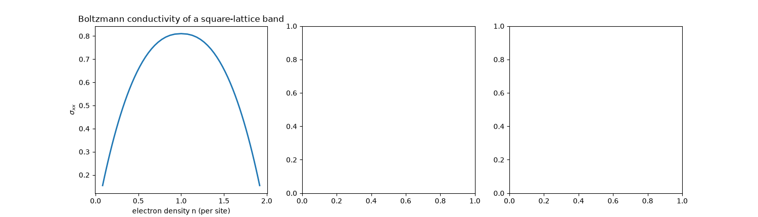
Text(0.5, 1.0, 'Boltzmann conductivity of a square-lattice band')

Wiedemann-Franz law

The Lorenz ratio is \(\pi^2/3\) for every filling, the universal Sommerfeld value. Drude’s classical theory gave \(3/2\) (and, with an error of a factor 2 in his original paper, roughly the measured value).

axes[1].plot(mus, lorenz, lw=2, label="Boltzmann, T = 0.02t")
axes[1].axhline(np.pi**2 / 3, color="k", ls="--", label=r"$\pi^2/3$ (Sommerfeld)")
axes[1].axhline(1.5, color="C3", ls=":", label="3/2 (classical Drude)")
axes[1].set_xlabel(r"chemical potential $\mu / t$")
axes[1].set_ylabel(r"$\kappa / \sigma T$")
axes[1].set_title("Lorenz number")
axes[1].set_ylim(1, 4)
axes[1].legend(fontsize=8)

<matplotlib.legend.Legend object at 0x370a85e20>

Mott formula for the thermopower

\(S = \frac{\pi^2 T}{3q}\frac{d\ln\sigma}{d\mu}\): small (of order \(T/E_F\)), and changing sign where the carriers change from electron-like to hole-like, at half filling.

mott = np.pi**2 * T / (3 * -1.0) * np.gradient(np.log(sigma), mus)
axes[2].plot(mus, seebeck, lw=2, label="Boltzmann")
axes[2].plot(mus, mott, "k--", lw=1, label="Mott formula")
axes[2].axhline(0, color="0.6", lw=0.5)
axes[2].set_xlabel(r"$\mu / t$")
axes[2].set_ylabel("Seebeck coefficient S")
axes[2].set_title("Thermopower changes sign at half filling")
axes[2].legend(fontsize=8)
fig.tight_layout()

Check

Wiedemann-Franz: L = pi^2/3 inside the band; the Mott formula matches the Boltzmann thermopower; S changes sign at half filling.

inside = np.abs(mus) < 3.0
np.testing.assert_allclose(lorenz[inside], np.pi**2 / 3, rtol=0.01)
assert np.max(np.abs(seebeck[inside] - mott[inside])) < 0.05 * np.max(np.abs(seebeck[inside]))
assert np.sign(seebeck[mus < -0.5][0]) == -np.sign(seebeck[mus > 0.5][-1])