A wave crossing a dielectric slab

Kane Yee’s staggered-grid update handles a wave crossing a material interface with no change to its core leapfrog rule – only the permittivity map eps_r fed into it changes: the TMz-mode Maxwell curl equations solved at every grid cell,

\[\frac{\partial H_x}{\partial t} = -\frac{1}{\mu_0}\frac{\partial E_z}{\partial y}, \qquad \frac{\partial H_y}{\partial t} = \frac{1}{\mu_0}\frac{\partial E_z}{\partial x}, \qquad \frac{\partial E_z}{\partial t} = \frac{1}{\varepsilon_0\varepsilon_r(x,y)}\left(\frac{\partial H_y}{\partial x} - \frac{\partial H_x}{\partial y}\right),\]

simply pick up a spatially varying \(\varepsilon_r(x,y)\) instead of the vacuum value 1. dielectric_slab() builds exactly such a map: vacuum everywhere except a slab (spanning grid columns i_start to i_end) of elevated permittivity eps_r_slab, so a broad Gaussian plane-wave pulse launched toward it partially reflects and partially refracts/transmits at each interface, exactly as an ordinary glass slab does to light.

import matplotlib.pyplot as plt
import numpy as np

from physicskit.fields import EPS0, MU0, animate_field_2d, courant_limit_2d, dielectric_slab, fdtd_2d_tmz_evolve

A broad plane-wave pulse launched toward a dielectric slab

Nx, Ny, dx, dy = 220, 60, 1e-3, 1e-3
dt = 0.5 * courant_limit_2d(dx, dy)
eta0 = np.sqrt(MU0 / EPS0)
x0, sigma = 40, 8

i = np.arange(Nx)
Ez0 = np.tile(np.exp(-((i - x0) ** 2) / (2 * sigma**2)), (Ny, 1)).T
ih = i + 0.5
Hy0 = np.tile(np.exp(-((ih - x0) ** 2) / (2 * sigma**2)) / eta0, (Ny, 1)).T
Hx0 = np.zeros((Nx, Ny))

i_start, i_end, eps_r_slab = 110, 160, 4.0
eps_r = dielectric_slab((Nx, Ny), i_start=i_start, i_end=i_end, eps_r_slab=eps_r_slab)
mu_r = np.ones((Nx, Ny))

Leapfrog the staggered E/H update forward, recording snapshots

steps = 420
frames, times = fdtd_2d_tmz_evolve(Ez0, Hx0, Hy0, eps_r, mu_r, steps=steps, dt=dt, dx=dx, dy=dy, snapshot_stride=6)

By the final frame, part of the pulse has reflected off the slab’s entrance interface (visible back in the vacuum region), and part has transmitted through and out the far side, at a speed slowed by \(1/\sqrt{\varepsilon_r}\) while inside the slab.

x = np.arange(Nx) * dx
y = np.arange(Ny) * dy
X, Y = np.meshgrid(x, y, indexing="ij")

anim = animate_field_2d(X, Y, frames, times)
plt.show()

To save the animation to a file instead of (or in addition to) displaying it interactively, use e.g.:

anim.save("dielectric_slab.gif", writer="pillow", fps=20)

reflected_region = frames[-1, : i_start - 20, Ny // 2]
transmitted_region = frames[-1, i_end + 5 :, Ny // 2]
fresnel_r = abs((1.0 - np.sqrt(eps_r_slab)) / (1.0 + np.sqrt(eps_r_slab)))
print(f"peak |Ez| reflected back into vacuum: {np.max(np.abs(reflected_region)):.4f}")
print(f"peak |Ez| transmitted past the slab: {np.max(np.abs(transmitted_region)):.4f}")
print(f"normal-incidence Fresnel |r| for eps_r={eps_r_slab}: {fresnel_r:.4f} (single-interface reference)")

peak |Ez| reflected back into vacuum: 0.7193
peak |Ez| transmitted past the slab: 0.0002
normal-incidence Fresnel |r| for eps_r=4.0: 0.3333 (single-interface reference)

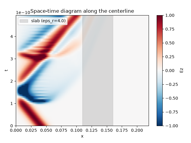
A space-time diagram along the beam axis

The animation shows the full 2D field but only one frame at a time; stacking the centerline (y = Ny//2) of every already-recorded snapshot into a single image shows the whole history at once: the incident pulse’s constant-slope (speed \(c_0\)) ridge, a reflected ridge peeling back off the slab’s entrance interface, and a visibly shallower-sloped ridge – moving at \(c_0/\sqrt{\varepsilon_r}\), half the vacuum speed for \(\varepsilon_r=4\) – still partway across the slab by the final recorded frame, not yet having reached the exit interface at this run’s steps.

centerline = frames[:, :, Ny // 2]
fig2, ax2 = plt.subplots()
extent = (x.min(), x.max(), times.min(), times.max())
im = ax2.imshow(centerline, extent=extent, origin="lower", aspect="auto", cmap="RdBu_r", vmin=-1, vmax=1)
ax2.axvspan(i_start * dx, i_end * dx, color="gray", alpha=0.25, label=f"slab (eps_r={eps_r_slab})")
fig2.colorbar(im, ax=ax2, label="Ez")
ax2.set_xlabel("x")
ax2.set_ylabel("t")
ax2.set_title("Space-time diagram along the centerline")
ax2.legend(loc="upper left")
fig2.tight_layout()