A Hertzian dipole antenna radiating on the Yee grid

Twenty-two years after Maxwell’s equations predicted electromagnetic radiation, Heinrich Hertz built an oscillating dipole antenna – an induction coil driving a spark gap – and detected the resulting waves meters away, confirming they travel at the speed of light and can be reflected, refracted, and polarized just like ordinary light. On the 2D Yee grid used here, the out-of-plane field \(E_z\) and the in-plane fields \(H_x\), \(H_y\) obey the source-free TMz-mode reduction of Maxwell’s curl equations,

\[\frac{\partial H_x}{\partial t} = -\frac{1}{\mu_0}\frac{\partial E_z}{\partial y}, \qquad \frac{\partial H_y}{\partial t} = \frac{1}{\mu_0}\frac{\partial E_z}{\partial x}, \qquad \frac{\partial E_z}{\partial t} = \frac{1}{\varepsilon_0}\left(\frac{\partial H_y}{\partial x} - \frac{\partial H_x}{\partial y}\right),\]

and oscillating_dipole_source() builds a soft point source – Hertz’s spark-gap transmitter, in miniature – that adds \(A\sin(2\pi f t)\) directly into \(E_z\) at a single grid cell every step, standing in for the driving antenna current. fdtd_2d_tmz_evolve() records the outgoing Ez field as it radiates away from the antenna on the Yee grid, frame by frame.

import matplotlib.pyplot as plt
import numpy as np

from physicskit.fields import animate_field_2d, courant_limit_2d, fdtd_2d_tmz_evolve, oscillating_dipole_source

An oscillating dipole source at the center of an empty 2D Yee grid – Hertz’s spark-gap transmitter, in miniature ————————————————————————

Nx, Ny, dx, dy = 100, 100, 1e-3, 1e-3
dt = 0.5 * courant_limit_2d(dx, dy)
Ez0 = np.zeros((Nx, Ny))
Hx0 = np.zeros((Nx, Ny))
Hy0 = np.zeros((Nx, Ny))
eps_r, mu_r = np.ones((Nx, Ny)), np.ones((Nx, Ny))
source = oscillating_dipole_source(Nx // 2, Ny // 2, amplitude=1.0, freq=3e10)

Record snapshots as the field radiates outward from the antenna

steps = 140
frames, times = fdtd_2d_tmz_evolve(Ez0, Hx0, Hy0, eps_r, mu_r, steps=steps, dt=dt, dx=dx, dy=dy, source=source, snapshot_stride=2)

Just as Hertz’s receiver detected sparks far from the transmitter, energy from the dipole has visibly spread across the grid as an outgoing circular wavefront by the final frame.

x = np.arange(Nx) * dx
y = np.arange(Ny) * dy
X, Y = np.meshgrid(x, y, indexing="ij")

anim = animate_field_2d(X, Y, frames, times)
plt.show()

To save the animation to a file instead of (or in addition to) displaying it interactively, use e.g.:

anim.save("dipole_radiation.gif", writer="pillow", fps=20)

radius_cells = frames.shape[1] // 2 - 5
outer_ring_energy = np.abs(frames[-1, radius_cells:, Ny // 2]).max()
print(f"peak |Ez| near the grid edge at the final frame: {outer_ring_energy:.4f} (radiation has arrived)")

peak |Ez| near the grid edge at the final frame: 0.5455 (radiation has arrived)

The radiation pattern at fixed radius, all the way around the antenna

The animation only shows the field along the grid; sampling the final Ez frame on a circle of fixed radius around the source, at every angle, shows the actual radiation pattern directly. This 2D TMz-mode soft source is a scalar point emitter, not a true 3D current-element dipole with directional lobes, so on a fine grid it would radiate isotropically; at the modest resolution used here (about 10 grid cells per wavelength), however, the square Yee grid’s own numerical dispersion is direction-dependent – waves travel at a very slightly different phase speed along the grid axes than along the diagonals – so the pattern instead comes out visibly fourfold-symmetric, a direct picture of that well-known low-order FDTD grid anisotropy rather than of any antenna directionality.

theta = np.linspace(0.0, 2.0 * np.pi, 360, endpoint=False)
i_theta = np.clip(np.round(Nx // 2 + radius_cells * np.cos(theta)).astype(int), 0, Nx - 1)
j_theta = np.clip(np.round(Ny // 2 + radius_cells * np.sin(theta)).astype(int), 0, Ny - 1)
pattern = np.abs(frames[-1, i_theta, j_theta])

fig2 = plt.figure()
ax2 = fig2.add_subplot(projection="polar")
ax2.plot(theta, pattern)
ax2.set_title(f"|Ez| at r = {radius_cells} cells, final frame\n(fourfold pattern: Yee-grid numerical anisotropy, not a directional antenna)")
fig2.tight_layout()

print(f"radiation pattern at fixed radius: min={pattern.min():.4f}, max={pattern.max():.4f}")
print("(the fourfold spread reflects FDTD grid anisotropy at this resolution, not true antenna directionality)")

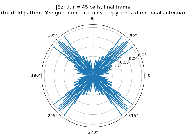
radiation pattern at fixed radius: min=0.0000, max=0.0504
(the fourfold spread reflects FDTD grid anisotropy at this resolution, not true antenna directionality)