A standing TM cavity mode oscillating in place

fdtd_2d_tmz() and fdtd_2d_tmz_evolve() integrate the same TMz-mode Maxwell curl equations as the other FDTD examples in this gallery, but already enforce Ez=0 on all four grid edges every step – exactly a perfectly-conducting (PEC) cavity wall, no absorbing boundary needed. A rectangular PEC cavity of size \(L_x\times L_y\) supports discrete standing-wave modes

\[E_z(x,y) = \sin\!\left(\frac{m\pi x}{L_x}\right)\sin\!\left(\frac{n\pi y}{L_y}\right), \qquad \omega_{mn} = c_0\pi\sqrt{\left(\frac{m}{L_x}\right)^2 + \left(\frac{n}{L_y}\right)^2},\]

which already vanish on the boundary by construction. tmz_cavity_mode() builds this analytic \(TM_{mn}\) mode shape directly; seeding the FDTD grid with it (here \(m=n=1\)) launches a mode that oscillates in place at its analytic frequency \(\omega_{mn}\), rather than propagating outward the way the point-source and dipole-antenna demos do.

import matplotlib.pyplot as plt
import numpy as np

from physicskit.fields import animate_field_2d, courant_limit_2d, fdtd_2d_tmz_evolve, tmz_cavity_mode

The analytic TM_11 mode of a rectangular PEC cavity

Nx, Ny, dx, dy = 61, 41, 1e-3, 1e-3
m, n = 1, 1
Ez0, omega_mn = tmz_cavity_mode((Nx, Ny), dx, dy, m=m, n=n)
Hx0 = np.zeros((Nx, Ny))
Hy0 = np.zeros((Nx, Ny))
eps_r, mu_r = np.ones((Nx, Ny)), np.ones((Nx, Ny))
dt = 0.4 * courant_limit_2d(dx, dy)

Leapfrog the cavity forward and record snapshots

period = 2 * np.pi / omega_mn
steps = int(1.2 * period / dt)
frames, times = fdtd_2d_tmz_evolve(Ez0, Hx0, Hy0, eps_r, mu_r, steps=steps, dt=dt, dx=dx, dy=dy, snapshot_stride=max(steps // 60, 1))

The mode’s spatial shape stays fixed – it does not propagate anywhere, since it already vanishes on all four PEC walls – and only its amplitude oscillates sinusoidally in time at the analytic frequency \(\omega_{mn} = c_0\pi\sqrt{(m/L_x)^2+(n/L_y)^2}\).

x = np.arange(Nx) * dx
y = np.arange(Ny) * dy
X, Y = np.meshgrid(x, y, indexing="ij")

anim = animate_field_2d(X, Y, frames, times)
plt.show()

To save the animation to a file instead of (or in addition to) displaying it interactively, use e.g.:

anim.save("cavity_mode.gif", writer="pillow", fps=20)

probe_i, probe_j = Nx // 3, Ny // 3
probe_series = frames[:, probe_i, probe_j]
predicted = Ez0[probe_i, probe_j] * np.cos(omega_mn * times)
print(f"TM_{m}{n} analytic frequency omega_mn = {omega_mn:.4e} rad/s")
print(f"max deviation of the FDTD-evolved probe point from the analytic standing wave: {np.max(np.abs(probe_series - predicted)):.2e}")

TM_11 analytic frequency omega_mn = 2.8298e+10 rad/s
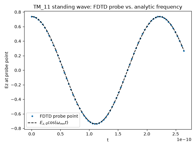
max deviation of the FDTD-evolved probe point from the analytic standing wave: 9.63e-03

The probe point’s time trace against the analytic standing wave

The animation shows the mode’s fixed spatial shape only oscillating in amplitude; plotting the FDTD-evolved probe point’s value against the analytic \(\cos(\omega_{mn}t)\) prediction directly, over the whole run, shows that oscillation tracking the exact frequency the cavity’s boundary conditions predict.

fig2, ax2 = plt.subplots()
ax2.plot(times, probe_series, "o", markersize=3, label="FDTD probe point")
ax2.plot(times, predicted, "k--", label=r"$E_{z,0}\cos(\omega_{mn}t)$")
ax2.set_xlabel("t")
ax2.set_ylabel("Ez at probe point")
ax2.set_title(f"TM_{m}{n} standing wave: FDTD probe vs. analytic frequency")
ax2.legend()
fig2.tight_layout()