Measuring the speed of light from Maxwell’s equations

James Clerk Maxwell unified electricity, magnetism, and optics into four coupled equations. In one dimension, source-free, they reduce to a coupled pair for the transverse electric and magnetic field components,

\[\frac{\partial H_y}{\partial t} = -\frac{1}{\mu_0}\frac{\partial E_z}{\partial x}, \qquad \frac{\partial E_z}{\partial t} = \frac{1}{\varepsilon_0}\frac{\partial H_y}{\partial x},\]

which combine into a wave equation admitting solutions propagating at \(c = 1/\sqrt{\varepsilon_0\mu_0}\) – matching the already-measured speed of light so closely that Maxwell concluded light itself is an electromagnetic wave. C0 is defined exactly this way, and fdtd_1d() solves the pair above on a Yee grid, verifying numerically that a propagating pulse moves at precisely this speed.

import matplotlib.pyplot as plt
import numpy as np

from physicskit.fields import C0, EPS0, MU0, courant_limit_1d, fdtd_1d, plot_field_1d

An impedance-matched Gaussian pulse: purely right-moving by construction

N, dx = 800, 1e-3
dt = 0.99 * courant_limit_1d(dx)
eta0 = np.sqrt(MU0 / EPS0)
x0, sigma = 100, 25
Ez0 = np.exp(-((np.arange(N) - x0) ** 2) / (2 * sigma**2))
xh = np.arange(N - 1) + 0.5
Hy0 = -np.exp(-((xh - x0) ** 2) / (2 * sigma**2)) / eta0  # right-moving: Hy = -Ez/eta0
eps_r, mu_r = np.ones(N), np.ones(N)

Integrate Maxwell’s equations on the Yee grid

steps = 360
Ez, Hy = fdtd_1d(Ez0, Hy0, eps_r, mu_r, steps=steps, dt=dt, dx=dx)

The pulse peak has moved at exactly \(c_0\) – Maxwell’s central prediction, verified directly by tracking the peak’s displacement.

measured_speed = (np.argmax(Ez) - x0) * dx / (steps * dt)

fig, ax = plot_field_1d(np.arange(N), Ez, label="Ez")
ax.set_title(f"measured speed / c0 = {measured_speed / C0:.4f}")
fig.tight_layout()

print(f"measured pulse speed / c0 = {measured_speed / C0:.6f}")

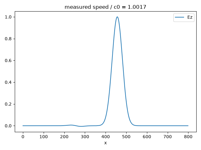
measured pulse speed / c0 = 1.001684

A space-time diagram: the pulse traces a single straight line

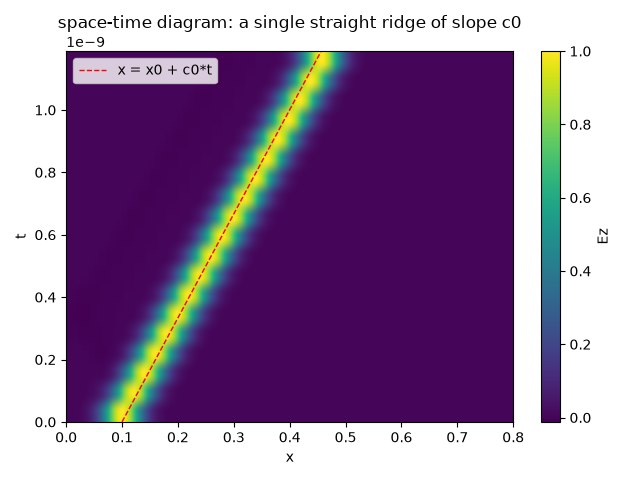
A single final-time snapshot only shows that the pulse arrived on time; re-running fdtd_1d() in short chunks (each chunk’s output fed back in as the next chunk’s initial condition – valid since it is a deterministic, one-step-at-a-time leapfrog integrator) and stacking every intermediate Ez snapshot into an image shows how: a rigid ridge of constant slope \(dx/dt = c_0\) the whole way across the grid, with no dispersive smearing or spreading.

n_snap_steps = 20
n_snapshots = steps // n_snap_steps
snapshots = np.empty((n_snapshots + 1, N))
snap_times = np.arange(n_snapshots + 1) * n_snap_steps * dt
Ez_s, Hy_s = Ez0.copy(), Hy0.copy()
snapshots[0] = Ez_s
for i in range(n_snapshots):
    Ez_s, Hy_s = fdtd_1d(Ez_s, Hy_s, eps_r, mu_r, steps=n_snap_steps, dt=dt, dx=dx)
    snapshots[i + 1] = Ez_s

fig2, ax2 = plt.subplots()
extent = (0, N * dx, snap_times[0], snap_times[-1])
im = ax2.imshow(snapshots, extent=extent, origin="lower", aspect="auto", cmap="viridis")
fig2.colorbar(im, ax=ax2, label="Ez")
ax2.plot([x0 * dx, x0 * dx + C0 * snap_times[-1]], [snap_times[0], snap_times[-1]], "r--", lw=1, label="x = x0 + c0*t")
ax2.set_xlabel("x")
ax2.set_ylabel("t")
ax2.set_title("space-time diagram: a single straight ridge of slope c0")
ax2.legend(loc="upper left")
fig2.tight_layout()