Berenger’s Perfectly Matched Layer vs. a hard wall

Jean-Pierre Berenger solved a problem that had limited FDTD simulations since Yee’s original 1966 paper: a finite grid needs some boundary condition, and a simple wall reflects outgoing waves right back into the simulation. His Perfectly Matched Layer (PML) is a graded absorbing medium whose wave impedance matches the interior exactly, so outgoing waves are absorbed rather than reflected. pml_conductivity_profile() implements a simplified (non-split-field) approximation to this idea: it grades an ordinary electric conductivity \(\sigma(x)\) smoothly up from zero over the outermost cells at each edge of the grid, so \(E_z\) there obeys the lossy telegraph-style update of a conducting medium rather than the lossless Ampere’s law,

\[\frac{\partial E_z}{\partial t} = \frac{1}{\varepsilon_0}\left(\frac{\partial H_y}{\partial x} - \sigma(x) E_z\right),\]

instead of a hard electric wall (\(E_z=0\)) that reflects everything outright. Comparing the two boundaries directly on the same launched pulse shows the dramatically smaller reflected echo the graded conductivity leaves behind.

import matplotlib.pyplot as plt
import numpy as np

from physicskit.fields import EPS0, MU0, courant_limit_1d, fdtd_1d, plot_field_1d, pml_conductivity_profile

A pulse launched toward the right boundary of a finite grid

N, dx = 500, 1e-3
dt = 0.99 * courant_limit_1d(dx)
eta0 = np.sqrt(MU0 / EPS0)
x0, sigma = 100, 10
Ez0 = np.exp(-((np.arange(N) - x0) ** 2) / (2 * sigma**2))
xh = np.arange(N - 1) + 0.5
Hy0 = -np.exp(-((xh - x0) ** 2) / (2 * sigma**2)) / eta0  # right-moving: Hy = -Ez/eta0
eps_r, mu_r = np.ones(N), np.ones(N)
steps = 900

Compare a hard (PEC) wall against Berenger’s graded-conductivity PML

Ez_wall, _ = fdtd_1d(Ez0.copy(), Hy0.copy(), eps_r, mu_r, steps=steps, dt=dt, dx=dx)
sigma_pml = pml_conductivity_profile(N, pml_width=120, dx=dx)
Ez_pml, _ = fdtd_1d(Ez0.copy(), Hy0.copy(), eps_r, mu_r, steps=steps, dt=dt, dx=dx, sigma=sigma_pml)

The PML leaves a far smaller reflected echo in the left half of the grid than the hard wall does – the same graded-impedance-matching idea behind Berenger’s original PML.

reflected_wall = np.max(np.abs(Ez_wall[: N // 2]))
reflected_pml = np.max(np.abs(Ez_pml[: N // 2]))

fig, ax = plot_field_1d(np.arange(N), Ez_wall, label="hard wall")
plot_field_1d(np.arange(N), Ez_pml, ax=ax, label="PML")
ax.set_title(f"reflected amplitude: wall={reflected_wall:.3f}, PML={reflected_pml:.3f}")
fig.tight_layout()

print(f"reflected amplitude, hard wall: {reflected_wall:.4f}")
print(f"reflected amplitude, PML:       {reflected_pml:.4f}")
print(f"reduction factor: {reflected_wall / reflected_pml:.1f}x")

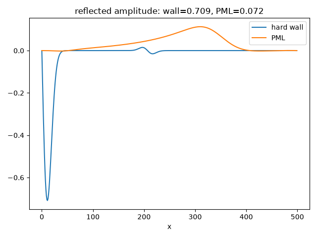
reflected amplitude, hard wall: 0.7088
reflected amplitude, PML:       0.0717
reduction factor: 9.9x

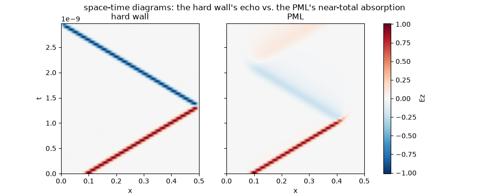
Space-time diagrams: the echo is a visible feature, not just a number

Re-running fdtd_1d() in short chunks (feeding each chunk’s output back in as the next chunk’s initial condition) and stacking the intermediate Ez snapshots into an image shows the reflected echo directly: a second ridge peeling off the right wall and heading back left in the hard-wall panel, barely visible at all in the PML panel.

n_snap_steps = 15
n_snapshots = steps // n_snap_steps
snap_times = np.arange(n_snapshots + 1) * n_snap_steps * dt


def _snapshot_series(sigma_profile):
    Ez_s, Hy_s = Ez0.copy(), Hy0.copy()
    snaps = np.empty((n_snapshots + 1, N))
    snaps[0] = Ez_s
    for i in range(n_snapshots):
        Ez_s, Hy_s = fdtd_1d(Ez_s, Hy_s, eps_r, mu_r, steps=n_snap_steps, dt=dt, dx=dx, sigma=sigma_profile)
        snaps[i + 1] = Ez_s
    return snaps


snaps_wall = _snapshot_series(None)
snaps_pml = _snapshot_series(sigma_pml)

fig2, (ax_wall, ax_pml) = plt.subplots(1, 2, figsize=(10, 4), sharey=True)
extent = (0, N * dx, snap_times[0], snap_times[-1])
vmax = max(np.abs(snaps_wall).max(), np.abs(snaps_pml).max())
for ax, snaps, title in ((ax_wall, snaps_wall, "hard wall"), (ax_pml, snaps_pml, "PML")):
    im = ax.imshow(snaps, extent=extent, origin="lower", aspect="auto", cmap="RdBu_r", vmin=-vmax, vmax=vmax)
    ax.set_xlabel("x")
    ax.set_title(title)
ax_wall.set_ylabel("t")
fig2.colorbar(im, ax=(ax_wall, ax_pml), label="Ez")
fig2.suptitle("space-time diagrams: the hard wall's echo vs. the PML's near-total absorption")

Text(0.5, 0.98, "space-time diagrams: the hard wall's echo vs. the PML's near-total absorption")