A point source radiating on the Yee grid

Kane Yee’s 1966 idea was deceptively simple: stagger the electric and magnetic field components on interleaved spatial and temporal grids (a “Yee cell”), so each field’s curl is naturally centered on the other’s location. fdtd_1d() and fdtd_2d_tmz() are direct implementations of this staggered-grid leapfrog scheme for the TMz-mode Maxwell curl equations,

\[\frac{\partial H_x}{\partial t} = -\frac{1}{\mu_0}\frac{\partial E_z}{\partial y}, \qquad \frac{\partial H_y}{\partial t} = \frac{1}{\mu_0}\frac{\partial E_z}{\partial x}, \qquad \frac{\partial E_z}{\partial t} = \frac{1}{\varepsilon_0}\left(\frac{\partial H_y}{\partial x} - \frac{\partial H_x}{\partial y}\right);\]

in 2D, a single grid cell of Ez set to 1 at \(t=0\) at the center of an otherwise empty grid then radiates outward as a circular wavefront, exactly as the Yee cell’s local update rule predicts for an isotropic medium.

import matplotlib.pyplot as plt
import numpy as np

from physicskit.fields import C0, courant_limit_2d, fdtd_2d_tmz, fdtd_2d_tmz_evolve, plot_poynting_field, poynting_vector_tmz

A point source at the center of an empty 2D Yee grid

Nx, Ny, dx, dy = 80, 80, 1e-3, 1e-3
dt = 0.5 * courant_limit_2d(dx, dy)
Ez0 = np.zeros((Nx, Ny))
Hx0 = np.zeros((Nx, Ny))
Hy0 = np.zeros((Nx, Ny))
eps_r, mu_r = np.ones((Nx, Ny)), np.ones((Nx, Ny))
Ez0[Nx // 2, Ny // 2] = 1.0

Leapfrog the staggered E/H update forward

steps = 25
Ez, Hx, Hy = fdtd_2d_tmz(Ez0, Hx0, Hy0, eps_r, mu_r, steps=steps, dt=dt, dx=dx, dy=dy)

Energy radiates outward as a circular wavefront of radius \(\sim c_0 t\) – the isotropic, second-order-accurate wave propagation that falls out of Yee’s staggered-grid update rule.

Sx, Sy = poynting_vector_tmz(Ez, Hx, Hy)
X, Y = np.meshgrid(np.arange(Nx), np.arange(Ny), indexing="ij")

fig, ax = plot_poynting_field(X, Y, Sx, Sy)
ax.set_title("Outward-radiating Poynting flux from a Yee-grid point source")
fig.tight_layout()

center = np.array([Nx // 2, Ny // 2])
flux_mag = np.sqrt(Sx**2 + Sy**2)
i, j = np.unravel_index(np.argmax(flux_mag), flux_mag.shape)
radius = np.hypot(i - center[0], j - center[1])
print(f"grid cell of peak outward energy flux: ({i}, {j}), radius from source = {radius:.1f} cells")

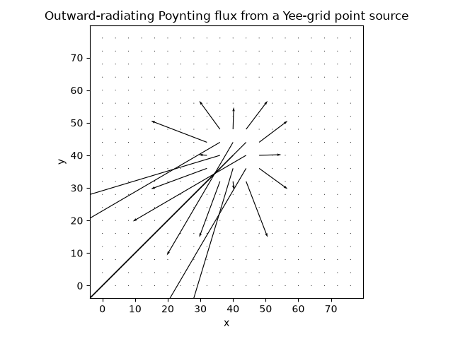
grid cell of peak outward energy flux: (37, 37), radius from source = 4.2 cells

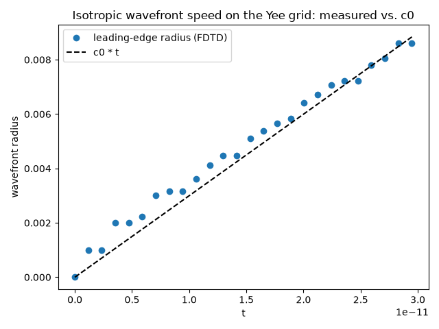
The wavefront radius grows (on average) at c0

The single final-time Poynting map above only shows where the flux is peaked at the end; recording every intermediate Ez snapshot with fdtd_2d_tmz_evolve() (the same solver, restructured only to also record history) and, at each recorded time, taking the farthest grid radius where |Ez| still exceeds a small fraction of its overall peak (the leading edge of the outgoing ring) shows how the wave got there, tracking the wavefront line \(r=c_0 t\) Yee’s staggered update rule predicts for a point source in vacuum – a single impulsive point source is not perfectly bandlimited, so this front tracking is noisier, cell-by-cell, than the smooth Gaussian pulses used elsewhere in this gallery.

frames, times = fdtd_2d_tmz_evolve(Ez0, Hx0, Hy0, eps_r, mu_r, steps=steps, dt=dt, dx=dx, dy=dy, snapshot_stride=1)
Xg, Yg = np.meshgrid(np.arange(Nx), np.arange(Ny), indexing="ij")
Rg = np.hypot(Xg - Nx // 2, Yg - Ny // 2) * dx
threshold = 0.05 * np.max(np.abs(frames[1:]))
front_radius = np.array([Rg[np.abs(frame) > threshold].max() if np.any(np.abs(frame) > threshold) else 0.0 for frame in frames])

fig2, ax2 = plt.subplots()
ax2.plot(times, front_radius, "o", label="leading-edge radius (FDTD)")
ax2.plot(times, C0 * times, "k--", label="c0 * t")
ax2.set_xlabel("t")
ax2.set_ylabel("wavefront radius")
ax2.set_title("Isotropic wavefront speed on the Yee grid: measured vs. c0")
ax2.legend()
fig2.tight_layout()