Relaxing to the Gross-Pitaevskii interacting ground state

Eugene Gross and Lev Pitaevskii independently derived, in 1961, a mean-field equation for the macroscopic wavefunction of a dilute Bose-Einstein condensate: a nonlinear Schrodinger equation with a cubic self-interaction term, \(i\hbar\partial_t\psi = [-\tfrac{\hbar^2}{2m}\nabla^2 + V + g|\psi|^2]\psi\). Decades before a real BEC existed in a laboratory, this gave theorists a concrete tool for its structure. In the natural units used here (\(\hbar=m=1\)) for a condensate held in a 2D harmonic trap \(V(\mathbf{r})=\tfrac12(x^2+y^2)\),

\[i\partial_t\psi = \Big[-\tfrac12\nabla^2 + V(\mathbf{r}) + g|\psi|^2\Big]\psi,\]

gpe_relax() solves exactly this equation via imaginary-time propagation (\(\tau=it\), renormalizing the norm after every step): substituting \(\tau=it\) turns the oscillatory Schrodinger-like evolution into a gradient-flow relaxation that drains energy from any initial state and settles it into a stationary point of the energy, starting here from a noninteracting Gaussian cloud. Repulsive interactions (\(g>0\)) visibly broaden the relaxed cloud past that starting Gaussian.

import matplotlib.pyplot as plt
import numpy as np

from physicskit.fields import gpe_energy, gpe_relax, harmonic_trap_grid, plot_bec_density

A harmonically trapped condensate with repulsive interactions g > 0

n, length, g = 64, 12.0, 4.0
X, Y, KX, KY, K2 = harmonic_trap_grid(n, length)
V = 0.5 * (X**2 + Y**2)
psi0 = np.exp(-0.5 * (X**2 + Y**2)).astype(complex)

Imaginary-time propagation relaxes psi0 to the interacting ground state

psi = gpe_relax(psi0, V, g, dtau=5e-4, steps=2000, X=X, Y=Y, K2=K2)

Repulsion broadens the cloud past the noninteracting Gaussian – the mean-field density profile Gross and Pitaevskii predicted, verified here by comparing the relaxed cloud’s radius against the trivial noninteracting case.

E = gpe_energy(psi, V, g, X, Y, K2)
dx = X[1, 0] - X[0, 0]
r2_interacting = np.sum((X**2 + Y**2) * np.abs(psi) ** 2) * dx * dx
r2_noninteracting = np.sum((X**2 + Y**2) * np.abs(psi0) ** 2) * dx * dx / (np.sum(np.abs(psi0) ** 2) * dx * dx)

fig, ax = plot_bec_density(X, Y, psi)
ax.set_title(f"interaction energy = {E['interaction']:.3f}")
fig.tight_layout()

print(f"interaction energy: {E['interaction']:.4f} (0 would mean no broadening)")
print(f"<r^2>: noninteracting Gaussian = {r2_noninteracting:.4f}, relaxed g={g} cloud = {r2_interacting:.4f}")

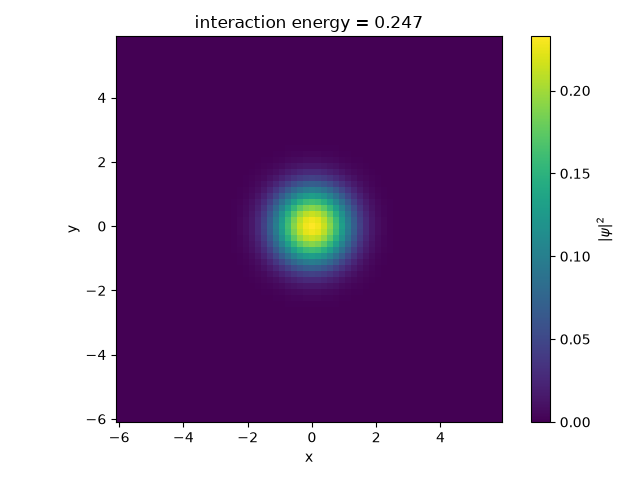
interaction energy: 0.2471 (0 would mean no broadening)
<r^2>: noninteracting Gaussian = 1.0000, relaxed g=4.0 cloud = 1.2451

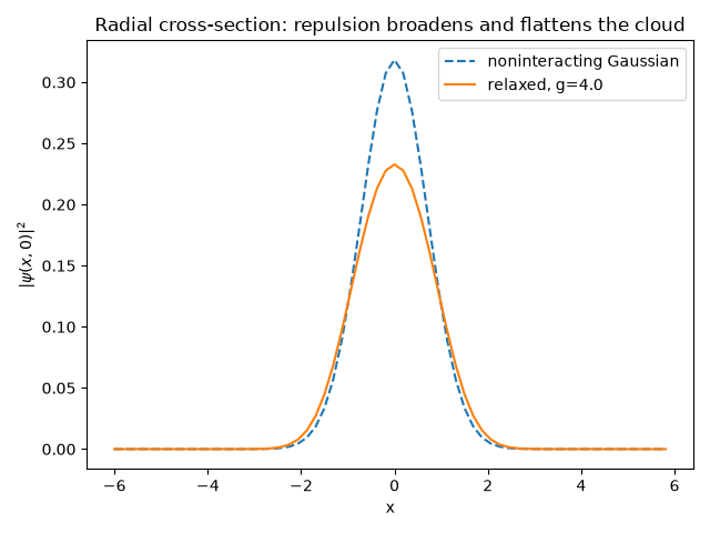
A radial cross-section makes the broadening directly visible

The 2D heatmap above shows the relaxed cloud’s shape, but only a cross-section through the trap center puts the interacting and noninteracting density profiles on the same axes, side by side, so the broadening summarized by <r^2> above is visible directly as a wider, flatter-topped profile – the Thomas-Fermi-like flattening repulsive interactions produce, in place of the noninteracting cloud’s pure Gaussian peak.

mid = n // 2
density_interacting = np.abs(psi[:, mid]) ** 2
density_noninteracting = np.abs(psi0[:, mid]) ** 2 / (np.sum(np.abs(psi0) ** 2) * dx * dx)

fig2, ax2 = plt.subplots()
ax2.plot(X[:, mid], density_noninteracting, "--", label="noninteracting Gaussian")
ax2.plot(X[:, mid], density_interacting, label=f"relaxed, g={g}")
ax2.set_xlabel("x")
ax2.set_ylabel(r"$|\psi(x, 0)|^2$")
ax2.set_title("Radial cross-section: repulsion broadens and flattens the cloud")
ax2.legend()
fig2.tight_layout()