A vortex genuinely precessing in real time

gpe_relax() only ever finds a stationary vortex state, by imaginary-time relaxation – it cannot show what a vortex actually does as time passes. gpe_evolve() solves the same Gross-Pitaevskii equation in genuine real (lab-frame) time instead,

\[i\partial_t\psi = \Big[-\tfrac12\nabla^2 + V(\mathbf{r}) + g|\psi|^2\Big]\psi \qquad (\hbar = m = 1),\]

with \(V(\mathbf{r}) = \tfrac12(x^2+y^2)\) the harmonic trap: seeded off-center in this trapped condensate, a single quantized vortex physically precesses around the trap center, driven by the local density gradient it sits in – the dynamical motion that, in a rotating condensate, carries a newly nucleated vortex into its place in the crystalline Abrikosov-like lattice.

import matplotlib.pyplot as plt
import numpy as np

from physicskit.fields import animate_density_2d, count_vortices, gpe_evolve, gpe_imprint_vortex, gpe_relax, harmonic_trap_grid

Relax a vortex-free ground state, then imprint one vortex off-center

n, length, g = 64, 14.0, 4.0
X, Y, KX, KY, K2 = harmonic_trap_grid(n, length)
V = 0.5 * (X**2 + Y**2)
psi_seed = np.exp(-0.5 * (X**2 + Y**2)).astype(complex)
psi_ground = gpe_relax(psi_seed, V, g, dtau=5e-4, steps=1500, X=X, Y=Y, K2=K2)
psi0 = gpe_imprint_vortex(psi_ground, X, Y, [(1.5, 0.0)])

Real-time propagation: the vortex is not held in place, it precesses

dt, steps, stride = 1e-3, 3000, 100
frames, times = gpe_evolve(psi0, V, g=g, dt=dt, steps=steps, K2=K2, snapshot_stride=stride)

Track the vortex core’s angular position frame by frame: it sweeps out a genuine orbit around the trap center rather than sitting still, the real-time dynamics gpe_relax() cannot show. An off-center vortex sits in a region where the background condensate density is already well below the trap’s peak density, so a lower-than-default density_threshold is needed to keep the vortex’s own (genuine, expected) local density dip from being masked out along with it.

detected_times, detected_angles = [], []
for t, frame in zip(times, frames):
    winding = count_vortices(frame, density_threshold=1e-3)
    if not np.any(winding):
        continue
    idx = np.unravel_index(np.argmax(np.abs(winding)), winding.shape)
    detected_times.append(t)
    detected_angles.append(np.arctan2(Y[idx], X[idx]))
detected_angles = np.unwrap(detected_angles)

extent = (X.min(), X.max(), Y.min(), Y.max())
anim = animate_density_2d(frames, extent=extent, times=times)
plt.show()

To save the animation to a file instead of (or in addition to) displaying it interactively, use e.g.:

anim.save("vortex_precession.gif", writer="pillow", fps=15)

print(
    f"vortex angular position: t={detected_times[0]:.2f} -> {np.degrees(detected_angles[0]):.1f} deg, "
    f"t={detected_times[-1]:.2f} -> {np.degrees(detected_angles[-1]):.1f} deg"
)
print(f"total angle swept (precession, not a stationary vortex): {np.degrees(detected_angles[-1] - detected_angles[0]):.1f} deg")

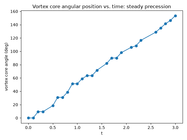
vortex angular position: t=0.00 -> 0.0 deg, t=3.00 -> 153.4 deg
total angle swept (precession, not a stationary vortex): 153.4 deg

The precession, plotted directly

The animation shows the vortex core drifting frame by frame, but only a plot of the already-detected core angle against time shows the actual precession rate directly: an essentially straight line (constant angular velocity), the signature of steady precession rather than random wandering or a decaying orbit.

fig2, ax2 = plt.subplots()
ax2.plot(detected_times, np.degrees(detected_angles), "o-")
ax2.set_xlabel("t")
ax2.set_ylabel("vortex core angle (deg)")
ax2.set_title("Vortex core angular position vs. time: steady precession")
fig2.tight_layout()