Self-focusing collapse of an attractive condensate

Vladimir Zakharov showed in “Collapse of Langmuir Waves” (1972) that the focusing nonlinear Schrodinger equation has a regime with no shape-preserving soliton at all: a sufficiently intense, narrow wave packet can self-focus so strongly that it contracts toward a genuine singularity in finite time, rather than settling into a stable envelope. gpe_evolve() solves the 2D Gross-Pitaevskii / cubic NLS equation

\[i\partial_t\psi = \Big[-\tfrac12\nabla^2 + V(\mathbf{r}) + g|\psi|^2\Big]\psi \qquad (\hbar = m = 1),\]

and, run here with no trapping potential (\(V=0\)) and an attractive interaction (\(g<0\), opposite sign convention from the 1D nls_evolve solver), reproduces exactly the runaway contraction of a sufficiently tall, narrow initial packet – the numerical, finite-grid stand-in for approaching (never reaching) Zakharov’s collapse; the calculation is stopped once the peak density is still visibly growing, not carried through the unresolvable blow-up itself.

import matplotlib.pyplot as plt
import numpy as np

from physicskit.fields import animate_density_2d, gpe_evolve, harmonic_trap_grid

A tall, narrow packet with attractive interactions and no trap

n, length = 64, 16.0
X, Y, KX, KY, K2 = harmonic_trap_grid(n, length)
V = np.zeros((n, n))
psi0 = 3.0 * np.exp(-0.5 * (X**2 + Y**2) / 0.5**2).astype(complex)

Real-time propagation under the attractive (g < 0) nonlinearity

dt, steps, stride = 2e-4, 400, 40
frames, times = gpe_evolve(psi0, V, g=-2.0, dt=dt, steps=steps, K2=K2, snapshot_stride=stride)

Peak density grows monotonically – self-focusing collapse, not a stable soliton, which would instead hold its peak density fixed as it propagates.

peak_density = np.max(np.abs(frames) ** 2, axis=(1, 2))

extent = (X.min(), X.max(), Y.min(), Y.max())
anim = animate_density_2d(frames, extent=extent, times=times)
plt.show()

To save the animation to a file instead of (or in addition to) displaying it interactively, use e.g.:

anim.save("self_focusing_collapse.gif", writer="pillow", fps=15)

print(f"peak density: t=0 -> {peak_density[0]:.3f}, t={times[-1]:.3f} -> {peak_density[-1]:.3f}")
print(f"density growth factor: {peak_density[-1] / peak_density[0]:.2f}x (a stable soliton would stay near 1.0x)")

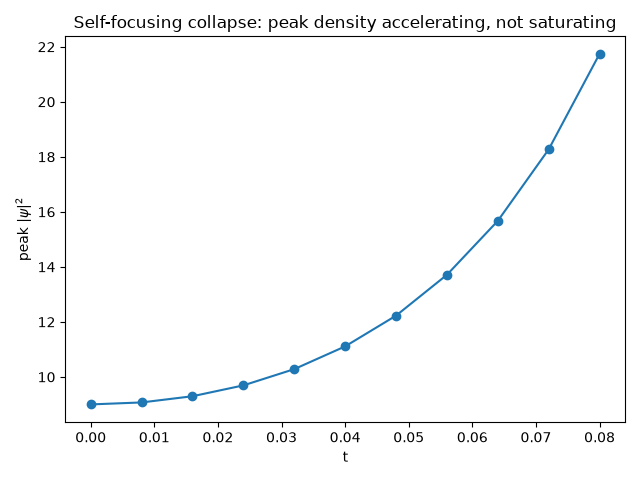
peak density: t=0 -> 9.000, t=0.080 -> 21.743
density growth factor: 2.42x (a stable soliton would stay near 1.0x)

Peak density over the whole run: runaway growth, not a plateau

The animation shows the packet visibly narrowing frame by frame, but plotting the already-recorded peak density against time directly shows the collapse accelerating – an ever-steepening curve, not the flat line a stable soliton (or the saturating curve of a process approaching some finite peak) would trace out.

fig2, ax2 = plt.subplots()
ax2.plot(times, peak_density, "o-")
ax2.set_xlabel("t")
ax2.set_ylabel(r"peak $|\psi|^2$")
ax2.set_title("Self-focusing collapse: peak density accelerating, not saturating")
fig2.tight_layout()