A bound vortex-antivortex pair: opposite windings that cancel at long range

John Kosterlitz and David Thouless explained how a two-dimensional superfluid can support order despite thermal fluctuations: below a critical temperature, vortices bind tightly into vortex-antivortex pairs of opposite circulation, whose combined velocity fields cancel at long range, leaving superfluid order intact; above it, the pairs unbind into a free plasma of independent vortices and antivortices. This package does not simulate the thermal binding-unbinding transition itself, but the two ingredients the picture is built from – an isolated vortex and its oppositely circulating antivortex – are both exactly representable as phase windings of a condensate wavefunction.

A single vortex, imprinted by gpe_imprint_vortex() as \((x-x_0)+i(y-y_0)\), carries a \(+2\pi\) phase winding; an antivortex carries the opposite, \(-2\pi\), winding, imprinted by the complex-conjugate factor \((x-x_0)-i(y-y_0)\) – the same construction with circulation reversed. count_vortices() detects both signs directly, as the \(\pm 1\) integer phase windings the Kosterlitz-Thouless picture pairs up (or unbinds): summed with their signs kept, the pair’s net winding is exactly zero at any loop enclosing both cores, the discrete signature of the canceling far-field the theory describes.

import matplotlib.pyplot as plt
import numpy as np

from physicskit.fields import count_vortices, gpe_imprint_vortex, harmonic_trap_grid, plot_bec_density, plot_bec_phase

Imprint one vortex and one antivortex, symmetric about the trap center

The vortex uses the same \((x-x_0)+i(y-y_0)\) winding factor as the single-vortex case above; the antivortex uses its complex conjugate, \((x-x_0)-i(y-y_0)\), the standard construction for a phase winding of opposite sign (Onsager 1949; Feynman 1955).

n, length = 64, 12.0
X, Y, KX, KY, K2 = harmonic_trap_grid(n, length)
psi0 = np.exp(-0.5 * (X**2 + Y**2) / 2.0**2).astype(complex)

separation = 2.0
x_vortex, x_antivortex = -separation / 2, separation / 2

dx = X[1, 0] - X[0, 0]
norm0 = np.sum(np.abs(psi0) ** 2) * dx * dx

psi_pair = gpe_imprint_vortex(psi0, X, Y, [(x_vortex, 0.0)])
# The antivortex is the complex-conjugate winding factor -- opposite
# circulation to gpe_imprint_vortex's own (x - x0) + i(y - y0) factor.
psi_pair = psi_pair * ((X - x_antivortex) - 1j * (Y - 0.0))
norm1 = np.sum(np.abs(psi_pair) ** 2) * dx * dx
psi_pair = psi_pair * np.sqrt(norm0 / norm1)

Detect both signed windings

count_vortices() reports a +1 at the vortex core and a -1 at the antivortex core – the same signed integers the Kosterlitz-Thouless picture pairs up below the transition.

# Two winding factors multiplying together (rather than just one, as in the
# single-vortex case above) suppress the density near *both* cores much more
# steeply relative to the field's new, higher far-field maximum, so the
# default 5%-of-max threshold masks out both real cores here; since this
# field is a smooth analytic product with no genuine numerical noise floor,
# a much smaller threshold recovers both without picking up anything else.
winding = count_vortices(psi_pair, density_threshold=1e-3)
net_winding = int(np.sum(winding))
total_cores = int(np.sum(np.abs(winding)))

print(f"total vortex cores detected: {total_cores} (expected: 2 -- one vortex, one antivortex)")
print(f"net signed winding, summed over both cores: {net_winding} (expected: 0 -- a bound, canceling pair)")

fig, (ax_density, ax_phase) = plt.subplots(1, 2, figsize=(10, 4))
plot_bec_density(X, Y, psi_pair, ax=ax_density)
ax_density.set_title(f"density: {total_cores} vortex cores")
plot_bec_phase(X, Y, psi_pair, ax=ax_phase)
ax_phase.set_title(f"phase: net winding = {net_winding}")
fig.tight_layout()

plt.show()

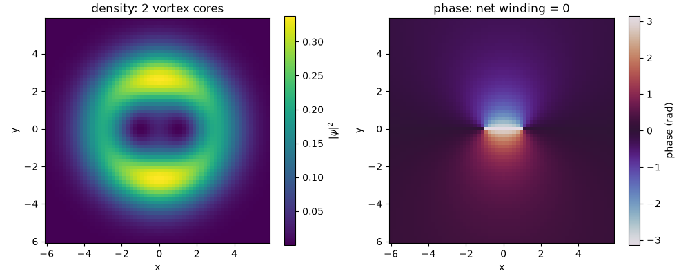
total vortex cores detected: 2 (expected: 2 -- one vortex, one antivortex)
net signed winding, summed over both cores: 0 (expected: 0 -- a bound, canceling pair)