An elastic KdV soliton-soliton collision

Korteweg and de Vries’s 1895 equation,

\[\partial_t u + 6 u\,\partial_x u + \partial_x^3 u = 0,\]

finally explained Russell’s wave mathematically – and revealed something stranger still: a fast, tall soliton overtaking a slower, shorter one passes straight through it, each recovering its exact original amplitude and speed afterward, merely phase-shifted. Here two exact kdv_soliton() humps of speed \(c=9\) and \(c=4\) (amplitude \(c/2\)) are launched on a periodic domain with the faster one trailing; propagating the sum forward with kdv_evolve() lets the fast soliton catch up to and pass through the slow one. This “elastic collision” is utterly unlike an ordinary nonlinear wave, which would break up or change shape on impact.

import matplotlib.pyplot as plt
import numpy as np
from scipy.signal import find_peaks

from physicskit.fields import kdv_evolve, kdv_evolve_frames, kdv_soliton, plot_field_1d

A fast, tall soliton launched behind a slower, shorter one

N, L = 512, 60.0
x = np.linspace(-L / 2, L / 2, N, endpoint=False)
u0 = kdv_soliton(x, c=9.0, x0=-20.0) + kdv_soliton(x, c=4.0, x0=-8.0)

The faster soliton overtakes and passes straight through the slower one

u = kdv_evolve(u0, x, dt=0.0005, steps=6000)

Elastic collision: both amplitudes survive completely unchanged (\(c/2\) = 4.5 and 2.0), only their positions are shifted.

peaks, _ = find_peaks(u, height=1.0)
surviving = sorted(round(float(h), 1) for h in u[peaks])

fig, ax = plot_field_1d(x, u0, label="t = 0")
plot_field_1d(x, u, ax=ax, label="after collision")
ax.set_title(f"surviving amplitudes: {surviving}")
fig.tight_layout()

print(f"surviving amplitudes after collision: {surviving} (expected [2.0, 4.5])")

surviving amplitudes after collision: [2.0, 4.5] (expected [2.0, 4.5])

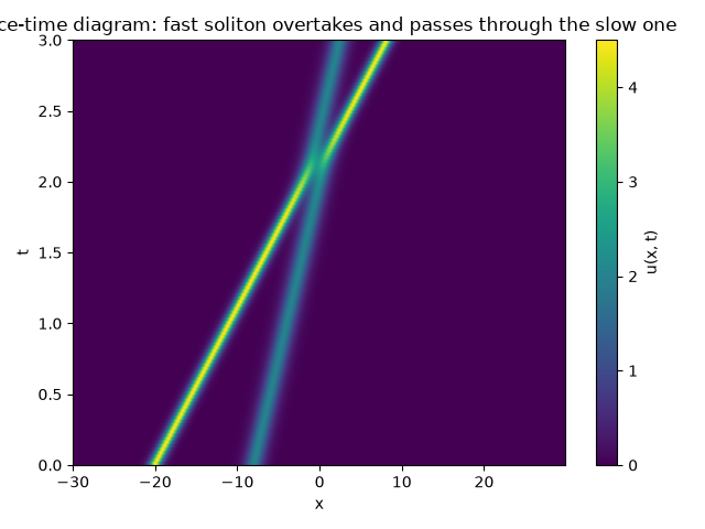
A space-time diagram: watching the pass-through itself

The before/after comparison above only shows the two endpoints; recording every intermediate snapshot with kdv_evolve_frames() (the same Strang-split integrator, restructured only to also keep a history) and stacking them into an image shows the actual collision: two ridges of different slope (speed) converging, visibly merging into one taller ridge as the fast soliton overtakes the slow one, then separating again afterward with each ridge’s slope unchanged – the elastic pass-through, not a mere before/after coincidence.

n_frames = 120
frames, times = kdv_evolve_frames(u0, x, dt=0.0005, steps_per_frame=6000 // n_frames, n_frames=n_frames)

fig2, ax2 = plt.subplots()
extent = (x.min(), x.max(), times.min(), times.max())
im = ax2.imshow(frames, extent=extent, origin="lower", aspect="auto", cmap="viridis")
fig2.colorbar(im, ax=ax2, label="u(x, t)")
ax2.set_xlabel("x")
ax2.set_ylabel("t")
ax2.set_title("Space-time diagram: fast soliton overtakes and passes through the slow one")
fig2.tight_layout()