Zabusky-Kruskal fission: coining “soliton”

Trying to resolve the Fermi-Pasta-Ulam-Tsingou recurrence puzzle, Norman Zabusky and Martin Kruskal simulated the continuum (KdV) limit of a nonlinear oscillator chain in 1965 and watched a single generic disturbance – not an exact multi-soliton solution – “fission” into a rank-ordered train of solitary waves that then collided and emerged unscathed. kdv_evolve() integrates the Korteweg-de Vries equation

\[\partial_t u + 6 u\,\partial_x u + \partial_x^3 u = 0\]

forward via a Strang-split pseudo-spectral scheme (the stiff linear dispersion \(\partial_x^3\) advanced exactly via the FFT, the non-stiff advection \(6u\partial_x u\) via RK4); started here from a plain Gaussian bump, \(u(x,0)=6\exp[-((x+15)/2)^2]\), rather than an exact soliton, it reproduces exactly this fission and gave the phenomenon its name, in direct analogy to a proton or electron.

import matplotlib.pyplot as plt
import numpy as np
from scipy.signal import find_peaks

from physicskit.fields import kdv_evolve, kdv_evolve_frames, plot_field_1d

A single generic bump – NOT an exact multi-soliton solution

N, L = 1024, 60.0
x = np.linspace(-L / 2, L / 2, N, endpoint=False)
u0 = 6.0 * np.exp(-(((x + 15) / 2.0) ** 2))

Zabusky and Kruskal’s numerical experiment: integrate KdV forward

u = kdv_evolve(u0, x, dt=0.0002, steps=8000)

The generic pulse fissions into a rank-ordered train of solitons plus dispersive radiation – the recurrence that inspired the name “soliton.”

peaks, _ = find_peaks(u, height=1.0)

fig, ax = plot_field_1d(x, u0, label="t = 0 (generic pulse)")
plot_field_1d(x, u, ax=ax, label="t > 0 (soliton train)")
ax.set_title(f"solitons resolved: {len(peaks)}")
fig.tight_layout()

print(f"single input bump fissioned into {len(peaks)} resolved solitary-wave peaks")
print(f"peak heights (rank-ordered by speed): {sorted(np.round(u[peaks], 2), reverse=True)}")

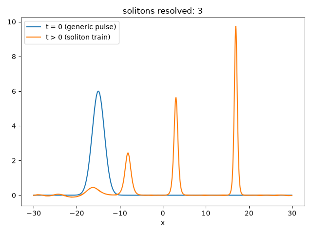
single input bump fissioned into 3 resolved solitary-wave peaks
peak heights (rank-ordered by speed): [np.float64(9.74), np.float64(5.63), np.float64(2.44)]

A space-time diagram of the fission itself

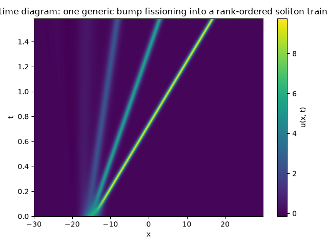
The before/after comparison above only shows the two endpoints; recording every intermediate snapshot with kdv_evolve_frames() (the same Strang-split integrator Zabusky and Kruskal would recognize, restructured only to also keep a history) and stacking them into an image shows the generic bump visibly splitting into rank-ordered ridges of increasing slope (the taller, faster solitons pulling ahead of the shorter, slower ones) plus a trailing wake of dispersive radiation – the “fission” Zabusky and Kruskal watched happen, frame by frame.

n_frames = 120
frames, times = kdv_evolve_frames(u0, x, dt=0.0002, steps_per_frame=8000 // n_frames, n_frames=n_frames)

fig2, ax2 = plt.subplots()
extent = (x.min(), x.max(), times.min(), times.max())
im = ax2.imshow(frames, extent=extent, origin="lower", aspect="auto", cmap="viridis")
fig2.colorbar(im, ax=ax2, label="u(x, t)")
ax2.set_xlabel("x")
ax2.set_ylabel("t")
ax2.set_title("Space-time diagram: one generic bump fissioning into a rank-ordered soliton train")
fig2.tight_layout()