The Biot-Savart law: a current loop and a finite solenoid

Weeks after Ørsted saw a compass needle swing beside a current-carrying wire in 1820, Jean-Baptiste Biot and Félix Savart measured how the magnetic force fell off with distance from a long wire. Laplace turned their result into a law for each small piece of wire:

\[d\mathbf B = \frac{\mu_0 I}{4\pi}\,\frac{d\boldsymbol\ell\times\hat{\mathbf r}}{r^2}.\]

Summing it over a closed loop gives the loop’s on-axis field \(\mu_0 I R^2/2(R^2+z^2)^{3/2}\). Stacking many loops into a solenoid gives a nearly uniform field \(\mu_0 n I\) inside, which falls to half that value at each end. biot_savart_field() integrates each straight piece of a polyline wire exactly. This example checks it against both closed forms and draws the field lines.

import matplotlib.pyplot as plt
import numpy as np

from physicskit.fields import (
    MU0,
    biot_savart_field,
    circular_loop_path,
    loop_axial_field,
    solenoid_axial_field,
    solenoid_path,
)

A single current loop

I, R = 1.0, 0.1
loop = circular_loop_path(R, n_segments=512)
z = np.linspace(-0.4, 0.4, 81)
axis = np.column_stack([0 * z, 0 * z, z])
B_loop = biot_savart_field(loop, axis, current=I)[:, 2]
print(f"loop center: B = {B_loop[40] * 1e6:.4f} uT, mu0 I / 2R = {MU0 * I / (2 * R) * 1e6:.4f} uT")
print(f"max relative error on the axis: {np.max(np.abs(B_loop / loop_axial_field(I, R, z) - 1)):.1e}")

loop center: B = 6.2833 uT, mu0 I / 2R = 6.2832 uT
max relative error on the axis: 2.3e-05

A finite solenoid

A helix of 40 turns, 5 cm in radius and 40 cm long. Inside, the field plateaus at \(\mu_0 n I\). Outside, the field lines close back around like those of a bar magnet.

Rs, Ls, N = 0.05, 0.4, 40
coil = solenoid_path(Rs, Ls, N, points_per_turn=48)
zs = np.linspace(-0.4, 0.4, 81)
B_sol = biot_savart_field(coil, np.column_stack([0 * zs, 0 * zs, zs]), current=I)[:, 2]
B_inf = MU0 * N / Ls * I
print(f"solenoid center: {B_sol[40] / B_inf:.4f} mu0 n I; at the end: {B_sol[60] / B_inf:.4f} mu0 n I")

xg = np.linspace(-0.15, 0.15, 61)
zg = np.linspace(-0.35, 0.35, 121)
XG, ZG = np.meshgrid(xg, zg)
plane = np.stack([XG, np.zeros_like(XG), ZG], axis=-1)
B_plane = biot_savart_field(coil, plane, current=I)

fig, axes = plt.subplots(1, 3, figsize=(16, 5))
axes[0].plot(z * 100, B_loop * 1e6, "o", ms=3, label="biot_savart_field")
axes[0].plot(z * 100, loop_axial_field(I, R, z) * 1e6, "k--", lw=1, label="closed form")
axes[0].set_xlabel("z (cm)")
axes[0].set_ylabel(r"$B_z$ ($\mu$T)")
axes[0].set_title("current loop, on axis")
axes[0].legend()

axes[1].plot(zs * 100, B_sol / B_inf, "o", ms=3, label="helix, Biot-Savart")
axes[1].plot(zs * 100, solenoid_axial_field(I, N, Rs, Ls, zs) / B_inf, "k--", lw=1, label="current sheet")
axes[1].axhline(0.5, color="gray", lw=0.6, ls=":")
axes[1].axvline(Ls / 2 * 100, color="gray", lw=0.6, ls=":")
axes[1].set_xlabel("z (cm)")
axes[1].set_ylabel(r"$B_z / \mu_0 n I$")
axes[1].set_title("finite solenoid, on axis")
axes[1].legend()

mag = np.linalg.norm(B_plane, axis=-1)
axes[2].streamplot(XG * 100, ZG * 100, B_plane[..., 0], B_plane[..., 2], color=np.log(mag), cmap="viridis", density=1.5, linewidth=0.8)
turns_z = coil[::48, 2] * 100
axes[2].plot(np.full_like(turns_z, Rs * 100), turns_z, "o", ms=2.5, color="firebrick")
axes[2].plot(np.full_like(turns_z, -Rs * 100), turns_z, "x", ms=2.5, color="royalblue")
axes[2].set_aspect("equal")
axes[2].set_xlabel("x (cm)")
axes[2].set_ylabel("z (cm)")
axes[2].set_title("solenoid field lines (xz plane)")
fig.tight_layout()
plt.show()

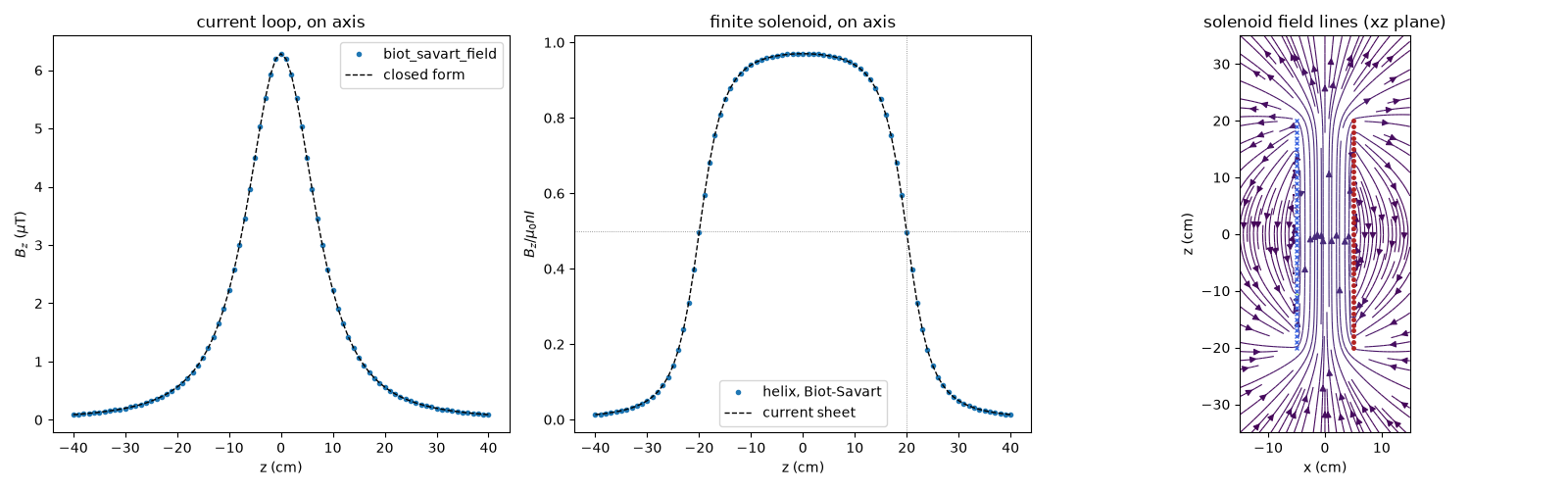
solenoid center: 0.9702 mu0 n I; at the end: 0.4961 mu0 n I

Check

Loop: B = mu0 I / 2R at the center. Finite solenoid on axis, in units of mu0 n I: (L/2) / sqrt(R^2 + L^2/4) at the center, L / (2 sqrt(R^2 + L^2)) at either end (just under half the infinite-solenoid value).

assert abs(B_loop[40] / (MU0 * I / (2 * R)) - 1) < 1e-4
assert np.max(np.abs(B_loop / loop_axial_field(I, R, z) - 1)) < 1e-4
assert abs(B_sol[40] / B_inf - (Ls / 2) / np.hypot(Rs, Ls / 2)) < 2e-3
assert abs(B_sol[60] / B_inf - Ls / (2 * np.hypot(Rs, Ls))) < 2e-3