Coulomb’s law: the inverse-square force and superposition

In 1785 Charles-Augustin de Coulomb hung a charged pith ball from a torsion balance and measured how the twist needed to hold a second charge at bay grew as he pushed them together. He found the electric force falls off as the inverse square of the distance,

\[\mathbf F = \frac{1}{4\pi\varepsilon_0}\frac{q_1 q_2}{r^2}\,\hat{\mathbf r},\]

the same law Newton had given for gravity. Because the law is linear in each charge, the field of any arrangement is the vector sum of the fields of its parts. coulomb_field() is exactly that sum. This example measures the exponent from a log-log fit and then builds the field lines of two charge pairs by superposition.

import matplotlib.pyplot as plt
import numpy as np

from physicskit.fields import EPS0, coulomb_field, coulomb_potential

Measuring the exponent

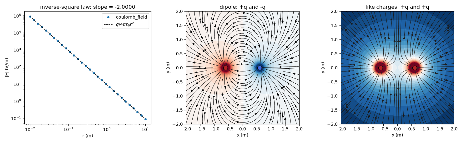
Coulomb’s balance data gave an exponent close to 2; Cavendish (1773, unpublished) and later null experiments pinned it to 2 within parts in \(10^{16}\). The field of a single 1 nC charge, sampled over three decades of distance, has slope exactly -2 on a log-log plot.

q = 1e-9
r = np.logspace(-2, 1, 30)
E = coulomb_field([q], [[0.0, 0.0, 0.0]], np.column_stack([r, 0 * r, 0 * r]))[:, 0]
slope = np.polyfit(np.log(r), np.log(E), 1)[0]
print(f"fitted exponent: {slope:.6f}")
E_1m = coulomb_field([q], [[0.0, 0.0, 0.0]], [[1.0, 0.0, 0.0]])[0, 0]
print(f"E at 1 m: {E_1m:.4f} V/m; q / (4 pi eps0 r^2) at 1 m = {q / (4 * np.pi * EPS0):.4f} V/m")

fitted exponent: -2.000000
E at 1 m: 8.9876 V/m; q / (4 pi eps0 r^2) at 1 m = 8.9876 V/m

Superposition: dipole and like charges

Two opposite charges give a dipole, whose field lines run from + to -. Two like charges give a saddle point halfway between them where the fields cancel.

x = np.linspace(-2, 2, 201)
X, Y = np.meshgrid(x, x)
grid = np.stack([X, Y], axis=-1)
pos = [[-0.6, 0.0], [0.6, 0.0]]

fig, axes = plt.subplots(1, 3, figsize=(15, 4.6))
axes[0].loglog(r, E, "o", ms=4, label="coulomb_field")
axes[0].loglog(r, q / (4 * np.pi * EPS0 * r**2), "k--", lw=1, label=r"$q/4\pi\varepsilon_0 r^2$")
axes[0].set_xlabel("r (m)")
axes[0].set_ylabel("|E| (V/m)")
axes[0].set_title(f"inverse-square law: slope = {slope:.4f}")
axes[0].legend()

for ax, charges, title in [(axes[1], [q, -q], "dipole: +q and -q"), (axes[2], [q, q], "like charges: +q and +q")]:
    field = coulomb_field(charges, pos, grid)
    phi = coulomb_potential(charges, pos, grid)
    mag = np.linalg.norm(field, axis=-1)
    ax.contourf(X, Y, np.clip(phi, -60, 60), levels=30, cmap="RdBu_r")
    ax.streamplot(X, Y, field[..., 0], field[..., 1], color=np.log(np.maximum(mag, 1e-3)), cmap="gray", density=1.4, linewidth=0.8)
    for (px, py), qi in zip(pos, charges):
        ax.plot(px, py, "o", ms=10, color="firebrick" if qi > 0 else "royalblue", mec="k")
    ax.set_aspect("equal")
    ax.set_title(title)
    ax.set_xlabel("x (m)")
    ax.set_ylabel("y (m)")
fig.tight_layout()

The like-charge saddle

Halfway between the two equal charges the fields cancel exactly, even though the potential there is not zero.

mid = coulomb_field([q, q], pos, [[0.0, 0.0]])[0]
print(f"field at the midpoint of two like charges: {np.linalg.norm(mid):.2e} V/m")
plt.show()

field at the midpoint of two like charges: 0.00e+00 V/m

Check

Coulomb: |E| = q / 4 pi eps0 r^2; like charges cancel at their midpoint.

assert abs(slope + 2) < 1e-9 and abs(E_1m - q / (4 * np.pi * EPS0)) < 1e-9 * E_1m
assert np.linalg.norm(mid) < 1e-9