Green’s function and the method of images

George Green’s 1828 Essay on the Application of Mathematical Analysis to the Theories of Electricity and Magnetism showed that the potential inside any region follows from a single function: the potential of a unit point charge that vanishes on the region’s boundary. Once you know this Green’s function, you can find the potential for any charge inside the region and any voltages on its boundary.

For a plane or a sphere the Green’s function can be written down directly. Place fictitious “image” charges outside the region so that the boundary becomes an equipotential (Thomson, 1847). This example uses image_charges_plane() and image_charges_sphere(). It checks that each conductor surface is an equipotential, that the induced surface charge integrates to the image charge, and that the force on the real charge is the Coulomb pull of its image.

import matplotlib.pyplot as plt
import numpy as np
from scipy.integrate import quad

from physicskit.fields import (
    EPS0,
    coulomb_field,
    coulomb_potential,
    image_charges_plane,
    image_charges_sphere,
    induced_charge_density_plane,
    induced_charge_density_sphere,
)

k = 1 / (4 * np.pi * EPS0)

A charge above a grounded plane

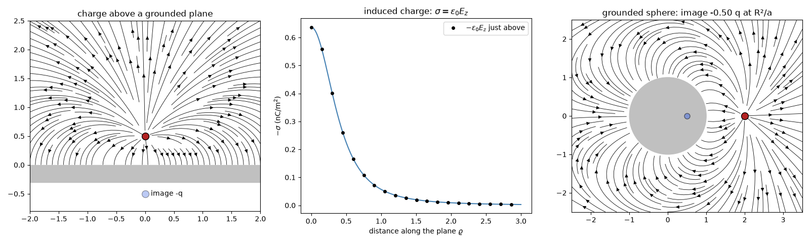
The image of \(q\) at height \(d\) is \(-q\) at \(-d\). The plane’s induced charge is \(\sigma = -qd/2\pi(\varrho^2 + d^2)^{3/2}\), which integrates to exactly \(-q\). The charge is pulled down with force \(q^2/(4\pi\varepsilon_0(2d)^2)\).

q, d = 1e-9, 0.5
qi, ri = image_charges_plane(q, [0.0, 0.0, d])
total, _ = quad(lambda s: induced_charge_density_plane(q, d, s) * 2 * np.pi * s, 0, np.inf)
F = q * coulomb_field(qi, ri, [0.0, 0.0, d])[2]
print(f"induced charge on the plane: {total:.4e} C   (-q = {-q:.4e} C)")
print(f"force on the charge: {F:.4e} N   (image law: {-k * q**2 / (2 * d) ** 2:.4e} N)")

induced charge on the plane: -1.0000e-09 C   (-q = -1.0000e-09 C)
force on the charge: -8.9876e-09 N   (image law: -8.9876e-09 N)

A charge outside a grounded sphere

For a sphere of radius \(R\) and a charge at distance \(a\), the image is \(-qR/a\) at \(R^2/a\). The induced charge on the sphere totals \(-qR/a\) rather than \(-q\). Some field lines escape to infinity.

R, a = 1.0, 2.0
qs, rs = image_charges_sphere(q, [a, 0.0, 0.0], R)
total_s, _ = quad(lambda th: induced_charge_density_sphere(q, a, R, th) * 2 * np.pi * R**2 * np.sin(th), 0, np.pi)
F_s = q * coulomb_field(qs, rs, [a, 0.0, 0.0])[0]
print(f"induced charge on the sphere: {total_s:.4e} C   (-qR/a = {-q * R / a:.4e} C)")
print(f"force: {F_s:.4e} N   (q^2 R a / 4 pi eps0 (a^2 - R^2)^2 = {-k * q**2 * R * a / (a**2 - R**2) ** 2:.4e} N)")
ang = np.linspace(0, 2 * np.pi, 400)
rim = np.column_stack([R * np.cos(ang), R * np.sin(ang), np.zeros_like(ang)])
rim_phi = coulomb_potential(np.r_[q, qs], np.vstack([[a, 0, 0], rs]), rim)
print(f"largest |potential| on the sphere: {np.max(np.abs(rim_phi)):.1e} V (grounded)")

induced charge on the sphere: -5.0000e-10 C   (-qR/a = -5.0000e-10 C)
force: -1.9972e-09 N   (q^2 R a / 4 pi eps0 (a^2 - R^2)^2 = -1.9972e-09 N)
largest |potential| on the sphere: 3.7e-15 V (grounded)

Field lines and induced charge

fig, axes = plt.subplots(1, 3, figsize=(16, 4.8))
x = np.linspace(-2, 2, 241)
Xp, Zp = np.meshgrid(x, np.linspace(0.001, 2.5, 151))
pts = np.stack([Xp, np.zeros_like(Xp), Zp], axis=-1)
Ep = coulomb_field(np.r_[q, qi], np.vstack([[0, 0, d], ri]), pts)
axes[0].streamplot(Xp, Zp, Ep[..., 0], Ep[..., 2], color="k", density=1.4, linewidth=0.6)
axes[0].axhspan(-0.3, 0, color="silver")
axes[0].plot(0, d, "o", color="firebrick", ms=10, mec="k")
axes[0].plot(0, -d, "o", color="royalblue", ms=10, mec="k", alpha=0.35)
axes[0].text(0.1, -d, "image -q", va="center")
axes[0].set_ylim(-0.8, 2.5)
axes[0].set_aspect("equal")
axes[0].set_title("charge above a grounded plane")

s = np.linspace(0, 3, 300)
axes[1].plot(s, -induced_charge_density_plane(q, d, s) * 1e9, color="steelblue")
eps0Ez = EPS0 * coulomb_field(np.r_[q, qi], np.vstack([[0, 0, d], ri]), np.column_stack([s[::15], 0 * s[::15], 0 * s[::15]]))[:, 2]
axes[1].plot(s[::15], -eps0Ez * 1e9, "o", ms=4, color="k", label=r"$-\varepsilon_0 E_z$ just above")
axes[1].set_xlabel(r"distance along the plane $\varrho$")
axes[1].set_ylabel(r"$-\sigma$ (nC/m$^2$)")
axes[1].set_title(r"induced charge: $\sigma = \varepsilon_0 E_z$")
axes[1].legend()

Xs, Ys = np.meshgrid(np.linspace(-2.5, 3.5, 241), np.linspace(-2.5, 2.5, 201))
pts = np.stack([Xs, Ys, np.zeros_like(Xs)], axis=-1)
outside = np.hypot(Xs, Ys) > R
Es = coulomb_field(np.r_[q, qs], np.vstack([[a, 0, 0], rs]), pts)
Es[~outside] = np.nan
axes[2].streamplot(Xs, Ys, Es[..., 0], Es[..., 1], color="k", density=1.4, linewidth=0.6)
axes[2].add_patch(plt.Circle((0, 0), R, color="silver"))
axes[2].plot(a, 0, "o", color="firebrick", ms=10, mec="k")
axes[2].plot(rs[0, 0], 0, "o", color="royalblue", ms=8, mec="k", alpha=0.5)
axes[2].set_aspect("equal")
axes[2].set_title(f"grounded sphere: image {qs[0] / q:+.2f} q at R²/a")
fig.tight_layout()
plt.show()

Check

Images: the plane carries induced charge -q and pulls with k q^2 / (2d)^2; the grounded sphere carries -qR/a, pulls with k q^2 R a / (a^2 - R^2)^2, and stays at zero potential.

assert abs(total / -q - 1) < 1e-6 and abs(F / (-k * q**2 / (2 * d) ** 2) - 1) < 1e-9
assert abs(total_s / (-q * R / a) - 1) < 1e-6 and abs(F_s / (-k * q**2 * R * a / (a**2 - R**2) ** 2) - 1) < 1e-9
assert np.max(np.abs(rim_phi)) < 1e-9