Young’s double-slit fringes

Thomas Young argued in his 1801 Bakerian Lecture that light passing through two closely spaced slits produces alternating bright and dark fringes on a distant screen, explicable only if light is a wave capable of constructive and destructive interference. Where the two path lengths from the slits to an observation point differ by an integer number of wavelengths the waves reinforce; where they differ by a half-integer number, they cancel. double_slit_aperture() builds exactly this two-slit transmission mask, and fraunhofer_diffraction() propagates it to the far field, reproducing Young’s fringe pattern directly from a computed intensity() distribution – no \(\sin\theta\) fringe formula is used, only the wave field itself. Rather than jumping straight to that far-field limit, animate_diffraction_propagation() animates the near-field wavefronts developing continuously into the far-field fringe pattern as the propagation distance grows.

import matplotlib.pyplot as plt
import numpy as np

from physicskit.optics.visualizers import animate_diffraction_propagation
from physicskit.optics.wave import double_slit_aperture, fraunhofer_diffraction, intensity

Two slits, propagated to the far field

wavelength = 0.5e-3  # mm
dx = 0.002
N = 512
width, separation = 0.01, 0.08
aperture = double_slit_aperture((N, N), dx=dx, width=width, separation=separation)

z = 500.0  # mm, far-field observation distance
U = fraunhofer_diffraction(aperture, wavelength=wavelength, z=z, dx=dx)
I = intensity(U)
x = (np.arange(N) - N // 2) * (wavelength * z / (N * dx))

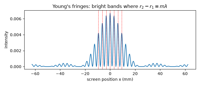
Fringe spacing: the interference maxima predicted by \(d\sin\theta = m\lambda\), at \(x_m \approx m\lambda z/d\) in the paraxial far field, compared against the bright fringes the propagated field actually produces.

fringe_spacing = wavelength * z / separation

fig, ax = plt.subplots(figsize=(7, 3))
ax.plot(x, I[N // 2])
for m in range(-3, 4):
    ax.axvline(m * fringe_spacing, color="r", ls="--", lw=0.7)
ax.set_xlabel("screen position x (mm)")
ax.set_ylabel("intensity")
ax.set_title(r"Young's fringes: bright bands where $r_2 - r_1 = m\lambda$")
fig.tight_layout()

peak_positions = x[N // 2 - 20 : N // 2 + 20][np.argmax(I[N // 2, N // 2 - 20 : N // 2 + 20])]
print(f"predicted fringe spacing lambda*z/d = {fringe_spacing:.4f} mm")
print(f"central maximum located at x = {peak_positions:.4f} mm (should be ~0)")

predicted fringe spacing lambda*z/d = 3.1250 mm
central maximum located at x = 0.0000 mm (should be ~0)

Watching the near field become the far field

Rather than a single far-field snapshot, sweep the propagation distance continuously and watch the two slits’ overlapping near-field wavefronts develop into Young’s far-field interference fringes.

aperture_complex = aperture.astype(complex)
z_values = np.geomspace(1.0, z, 40)

anim = animate_diffraction_propagation(aperture_complex, wavelength=wavelength, z_values=z_values, dx=dx, log_scale=True)
plt.show()

To save the animation to a file instead of (or in addition to) displaying it interactively, use e.g.:

anim.save("young_double_slit_propagation.gif", writer="pillow", fps=15)