Maxwell’s electromagnetic theory of light

Maxwell (1865) found that his field equations admit waves travelling at \(c = 1/\sqrt{\mu_0\varepsilon_0}\), a speed fixed by two constants measured with capacitors and coils, and that it matched the measured speed of light. Light, he concluded, is an electromagnetic wave. This example checks three consequences:

1. \(1/\sqrt{\mu_0\varepsilon_0}\) from physicskit.constants is the speed of light;

2. a pulse obtained by stepping Faraday’s and Ampère’s laws, \(\partial_t B = -\partial_x E\) and \(\varepsilon\,\partial_t E = -\mu_0^{-1}\partial_x B\) (a 1D Yee scheme), moves at \(c\) in vacuum and \(c/n\) in glass, and reflects from the glass with Fresnel’s amplitude \((1-n)/(1+n)\), here derived from field continuity alone;

3. the scalar Helmholtz equation that follows for one field component, solved by angular_spectrum_propagate(), spreads a Gaussian beam exactly as \(w(z)=w_0\sqrt{1+(z/z_R)^2}\).

import matplotlib.pyplot as plt
import numpy as np

from physicskit.constants import VACUUM_PERMEABILITY, VACUUM_PERMITTIVITY, C
from physicskit.optics.wave import angular_spectrum_propagate, field_grid

The speed of electromagnetic waves

c_maxwell = 1.0 / np.sqrt(VACUUM_PERMEABILITY * VACUUM_PERMITTIVITY)
print(f"1/sqrt(mu0 eps0) = {c_maxwell:,.1f} m/s")
print(f"speed of light c = {C:,.1f} m/s")

1/sqrt(mu0 eps0) = 299,792,458.0 m/s
speed of light c = 299,792,458.0 m/s

A light pulse from Maxwell’s equations

Fields in units where \(c=1\), with \(H\) scaled by the vacuum impedance so that \(E=H\) in a right-moving vacuum wave. At Courant number 1 the vacuum update is exact: the pulse moves one cell per step. A glass slab (\(n=2\)) occupies the right half.

N, n_glass = 1600, 2.0
x = np.arange(N)
eps_r = np.where(x >= 800, n_glass**2, 1.0)
E = np.exp(-(((x - 300) / 25.0) ** 2))
# H lives half a cell right of E and half a step later; for a right-moving
# pulse E = H = f(x - t), so H(x + 1/2, t = 1/2) = f(x).
H = E.copy()

snapshots = {}
for step in range(901):
    if step in (0, 400, 900):
        snapshots[step] = E.copy()
    E[1:] -= (H[1:] - H[:-1]) / eps_r[1:]  # Ampere
    H[:-1] -= E[1:] - E[:-1]  # Faraday

peak_400 = np.argmax(snapshots[400])
print(f"\nvacuum: pulse moved {peak_400 - 300} cells in 400 steps  (speed = c)")
E_final = snapshots[900]
i_refl = np.argmin(E_final[:800])
i_trans = 800 + np.argmax(E_final[800:])
print(f"glass:  transmitted pulse moved {i_trans - 800} cells in the {900 - 500} steps after entering (speed = c/{400 / (i_trans - 800):.3f})")
print(f"reflected amplitude   {E_final[i_refl]:+.4f}   Fresnel (1-n)/(1+n) = {(1 - n_glass) / (1 + n_glass):+.4f}")
print(f"transmitted amplitude {E_final[i_trans]:+.4f}   Fresnel 2/(1+n)     = {2 / (1 + n_glass):+.4f}")

fig1, ax1 = plt.subplots(figsize=(8, 3.8))
for (step, e), color in zip(snapshots.items(), ["0.6", "steelblue", "firebrick"]):
    ax1.plot(x, e, color=color, label=f"step {step}")
ax1.axvspan(800, N, color="lightblue", alpha=0.3, label=f"glass, n = {n_glass}")
ax1.set_xlabel("position [cells]")
ax1.set_ylabel("E")
ax1.set_title("A pulse from Faraday + Ampère: speed c, then c/n, partial reflection")
ax1.legend(fontsize=8, loc="upper left")
fig1.tight_layout()

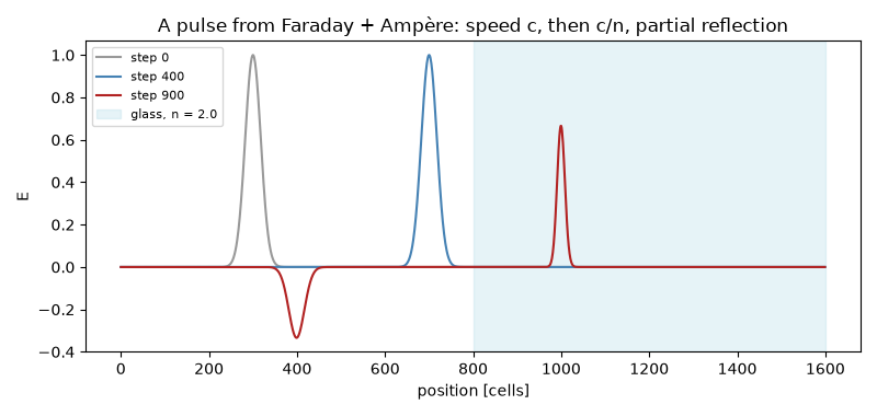
vacuum: pulse moved 400 cells in 400 steps  (speed = c)
glass:  transmitted pulse moved 200 cells in the 400 steps after entering (speed = c/2.000)
reflected amplitude   -0.3339   Fresnel (1-n)/(1+n) = -0.3333
transmitted amplitude +0.6657   Fresnel 2/(1+n)     = +0.6667

The Helmholtz equation: diffraction of a Gaussian beam

For one monochromatic field component, Maxwell’s wave equation becomes \((\nabla^2+k^2)E=0\). Its exact plane-wave solution, the angular spectrum method, spreads a Gaussian beam of waist \(w_0\) over the Rayleigh range \(z_R=\pi w_0^2/\lambda\).

wavelength, w0, dx = 633e-9, 50e-6, 4e-6
X, Y = field_grid((256, 256), dx)
U0 = np.exp(-(X**2 + Y**2) / w0**2)
z_R = np.pi * w0**2 / wavelength
z_values = np.linspace(0, 4 * z_R, 9)
w_numeric = []
for z in z_values:
    I = np.abs(angular_spectrum_propagate(U0, wavelength, z, dx)) ** 2
    w_numeric.append(2 * np.sqrt(np.sum(X**2 * I) / np.sum(I)))  # 1/e^2 radius = 2 * rms width
w_numeric = np.array(w_numeric)
w_theory = w0 * np.sqrt(1 + (z_values / z_R) ** 2)
print(f"\nGaussian beam: max |w_numeric / w_theory - 1| = {np.max(np.abs(w_numeric / w_theory - 1)):.1e}")

fig2, ax2 = plt.subplots(figsize=(5.5, 3.8))
ax2.plot(z_values * 1e3, w_numeric * 1e6, "o", color="steelblue", label="angular spectrum (Helmholtz)")
ax2.plot(z_values * 1e3, w_theory * 1e6, "--", color="orange", label=r"$w_0\sqrt{1+(z/z_R)^2}$")
ax2.set_xlabel("z [mm]")
ax2.set_ylabel("beam radius w [µm]")
ax2.set_title("Scalar diffraction from Maxwell's wave equation")
ax2.legend(fontsize=8)
fig2.tight_layout()

plt.show()

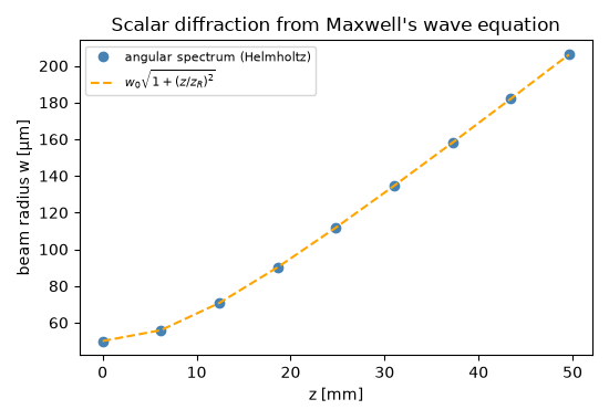
Gaussian beam: max |w_numeric / w_theory - 1| = 7.5e-06

Check

c = 1/sqrt(mu0 eps0); the Yee pulse moves at c in vacuum and c/n in glass, with Fresnel amplitudes (1 - n)/(1 + n) and 2/(1 + n); the Gaussian beam spreads as w0 sqrt(1 + (z/zR)^2).

assert abs(c_maxwell / C - 1) < 1e-9
assert peak_400 - 300 == 400 and i_trans - 800 == 200
assert abs(E_final[i_refl] - (1 - n_glass) / (1 + n_glass)) < 0.005
assert abs(E_final[i_trans] - 2 / (1 + n_glass)) < 0.005
assert np.max(np.abs(w_numeric / w_theory - 1)) < 1e-4