Huygens’ wavelets: diffractive spreading of a pinhole

Christiaan Huygens’ 1690 construction treats every point of an advancing wavefront as the source of a new spherical secondary wavelet; the envelope of all those wavelets a moment later reconstructs the propagated wavefront. angular_spectrum_propagate() realizes exactly this modern form of the picture. The scalar field \(U_0(x,y)\) right after the aperture is decomposed into its plane-wave (angular) spectrum by a 2D Fourier transform; each plane-wave component, labeled by transverse spatial frequency \((f_x,f_y)\), is a secondary wavelet that advances rigidly along \(z\) picking up phase \(e^{ik_z z}\); re-synthesizing (inverse Fourier transform) sums the interference of all these wavelets at the new plane:

\[\begin{split}U(x,y;z) = \mathcal{F}^{-1}\!\left[ \mathcal{F}[U_0](f_x,f_y)\; e^{ik_z z} \right], \qquad k_z = \begin{cases} \sqrt{k^2 - k_x^2 - k_y^2} & k_x^2+k_y^2 \le k^2 \quad \text{(propagating)}\\ i\sqrt{k_x^2+k_y^2 - k^2} & k_x^2+k_y^2 > k^2 \quad \text{(evanescent)} \end{cases}\end{split}\]

with \(k=2\pi/\lambda\), \(k_x=2\pi f_x\), \(k_y=2\pi f_y\). Because this sums the exact plane-wave spectrum rather than a paraxial approximation, it is Huygens’ interference picture computed with no approximation beyond the scalar-wave treatment of light itself. A circular pinhole of radius radius = 0.01 mm – a few wavelengths across at wavelength = 0.5e-3 mm – makes an especially clean demonstration, since ray optics alone would predict a sharp-edged shadow of the aperture at every distance \(z\), while Huygens’ picture predicts the diffractive spreading seen below as \(z\) grows from 0.05 mm to 2.0 mm.

import matplotlib.pyplot as plt

from physicskit.optics.visualizers import plot_diffraction_pattern
from physicskit.optics.wave import angular_spectrum_propagate, circular_aperture

A pinhole a few wavelengths across: an array of Huygens point sources

wavelength = 0.5e-3  # mm
dx = 0.002  # mm per pixel
radius = 0.01  # mm
aperture = circular_aperture((256, 256), dx=dx, radius=radius).astype(complex)

Every open pixel re-radiates a spherical wavelet; angular_spectrum_propagate sums their interference at each successive plane – Huygens’ principle, computed exactly rather than approximated.

U_near = angular_spectrum_propagate(aperture, wavelength=wavelength, z=0.05, dx=dx)
U_far = angular_spectrum_propagate(aperture, wavelength=wavelength, z=2.0, dx=dx)

fig, axes = plt.subplots(1, 2, figsize=(10, 4.5))
plot_diffraction_pattern(U_near, dx=dx, ax=axes[0])
plot_diffraction_pattern(U_far, dx=dx, ax=axes[1])
axes[0].set_title("z = 0.05 mm\nclose to the aperture's geometric shadow", fontsize=10)
axes[1].set_title("z = 2.0 mm\ndiffractive spreading well beyond the shadow", fontsize=10)
fig.tight_layout()

print(f"aperture radius: {radius} mm, wavelength: {wavelength} mm")
print("the far-field pattern has spread well past the aperture's geometric")
print("shadow -- exactly what Huygens' wavelet construction predicts and")
print("plain ray optics cannot explain.")

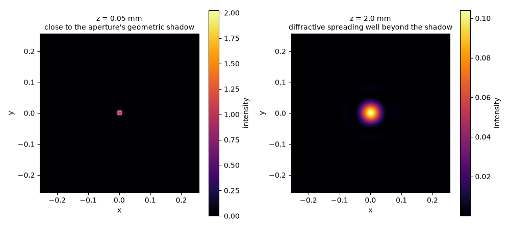
aperture radius: 0.01 mm, wavelength: 0.0005 mm
the far-field pattern has spread well past the aperture's geometric
shadow -- exactly what Huygens' wavelet construction predicts and
plain ray optics cannot explain.