Kogelnik and Li: focusing a Gaussian beam through a thin lens

After Maiman’s laser it became clear that real laser beams are neither idealized geometric rays nor infinite plane waves, but Gaussian beams. Kogelnik and Li’s 1966 paper showed that a Gaussian beam is completely characterized by one complex beam parameter \(q(z)\), and, crucially, that \(q\) transforms through any sequence of lenses, mirrors, or free-space sections by the same ABCD ray-transfer matrix already used for geometric rays – unifying ray optics and Gaussian-beam wave optics under one formalism. propagate_q() implements \(q' = (Aq+B)/(Cq+D)\), and q_to_beam_params() recovers the physical beam radius \(w(z)\) at any plane.

import matplotlib.pyplot as plt
import numpy as np

from physicskit.optics.gaussian import GaussianBeam, propagate_q, q_to_beam_params
from physicskit.optics.ray import free_space, thin_lens

A collimated-ish beam launched at its waist, focused through a thin lens

wavelength = 0.5e-3
beam = GaussianBeam(wavelength=wavelength, w0=1.0, z0=0.0)
f, d1 = 0.2, 1.0  # lens focal length, distance from source waist to lens

q0 = beam.q_parameter(d1)  # beam parameter just before the lens
q_after_lens = propagate_q(q0, thin_lens(f))

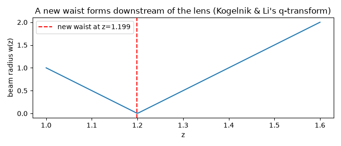
Kogelnik and Li’s q-transform: the same ABCD matrices used for ray tracing propagate the complex beam parameter, and a new waist forms downstream of the lens exactly where \(\mathrm{Re}(1/q) = 0\).

z2 = np.linspace(0.0, 0.6, 200)
w_after = np.array([q_to_beam_params(propagate_q(q_after_lens, free_space(z)), wavelength)[0] for z in z2])

fig, ax = plt.subplots(figsize=(7, 3))
ax.plot(d1 + z2, w_after)
new_waist_z = -q_after_lens.real  # q is purely imaginary at the waist
w_new = q_to_beam_params(propagate_q(q_after_lens, free_space(new_waist_z)), wavelength)[0]
ax.axvline(d1 + new_waist_z, color="r", ls="--", label=f"new waist at z={d1 + new_waist_z:.3f}")
ax.set_xlabel("z")
ax.set_ylabel("beam radius w(z)")
ax.legend()
ax.set_title("A new waist forms downstream of the lens (Kogelnik & Li's q-transform)")
fig.tight_layout()

print(f"source waist w0={beam.w0}, Rayleigh range zR={beam.rayleigh_range:.4f}")
print(f"lens focal length f={f} at distance d1={d1} from the source waist")
print(f"new waist radius: {w_new:.3e}, located {new_waist_z:.6f} past the lens")

source waist w0=1.0, Rayleigh range zR=6283.1853
lens focal length f=0.2 at distance d1=1.0 from the source waist
new waist radius: 3.183e-05, located 0.200000 past the lens

The full beam caustic: a 2D intensity map through the whole system

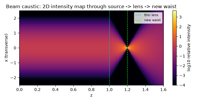
Rather than only the 1D envelope w(z) after the lens, stitch together the beam radius before the lens (waist()) and after it (the q-transform above) into one continuous w(z) over the full source -> lens -> new-waist path, and use it to build the 2D transverse Gaussian intensity profile \(I(x,z) \propto (w_0/w(z))^2 \exp[-2x^2/w(z)^2]\) at every plane – the beam “caustic” that a real focusing Gaussian beam traces out, showing the input beam narrowing into the lens and re-focusing to the new waist beyond it.

z1 = np.linspace(0.0, d1, 150)
w1 = beam.waist(z1)
z_full = np.concatenate([z1, d1 + z2[1:]])
w_full = np.concatenate([w1, w_after[1:]])

x_transverse = np.linspace(-2.5, 2.5, 400)
X_grid, _ = np.meshgrid(x_transverse, z_full)
I_caustic = (beam.w0 / w_full[:, None]) ** 2 * np.exp(-2.0 * X_grid**2 / w_full[:, None] ** 2)
log_I_caustic = np.log10(I_caustic + 1e-8 * I_caustic.max())

fig2, ax2 = plt.subplots(figsize=(7, 3.5))
im = ax2.pcolormesh(z_full, x_transverse, log_I_caustic.T, shading="auto", cmap="inferno", vmin=-4, vmax=np.log10(I_caustic.max()))
fig2.colorbar(im, ax=ax2, label="log10 relative intensity")
ax2.axvline(d1, color="c", ls="--", lw=1, label="thin lens")
ax2.axvline(d1 + new_waist_z, color="lime", ls="--", lw=1, label="new waist")
ax2.set_xlabel("z")
ax2.set_ylabel("x (transverse)")
ax2.legend(fontsize=8, loc="upper right")
ax2.set_title("Beam caustic: 2D intensity map through source -> lens -> new waist")
fig2.tight_layout()

Check

Kogelnik’s thin-lens waist transform: w0’ = w0 f / sqrt((d1 - f)^2 + zR^2) at z’ = f + (d1 - f) f^2 / ((d1 - f)^2 + zR^2) past the lens – for a source this far inside its Rayleigh range, essentially the focal point.

zR = beam.rayleigh_range
denominator = (d1 - f) ** 2 + zR**2
assert abs(w_new / (beam.w0 * f / np.sqrt(denominator)) - 1) < 1e-9
assert abs(new_waist_z - (f + (d1 - f) * f**2 / denominator)) < 1e-12
assert np.all(w_after >= w_new)