Siegman’s \(M^2\) beam-quality factor

Real laser beams are never perfectly diffraction-limited fundamental Gaussian modes: multimode content, aberrations, and gain-medium imperfections all make them diverge faster than an ideal beam of the same waist. Anthony Siegman showed that essentially every real laser beam’s second-moment width still propagates by the same functional form as an ideal Gaussian beam,

\[w(z) = w_0 \sqrt{1 + \left(\frac{z}{z_{R,\text{eff}}}\right)^2}, \qquad z_{R,\text{eff}} = \frac{\pi w_0^2}{M^2 \lambda},\]

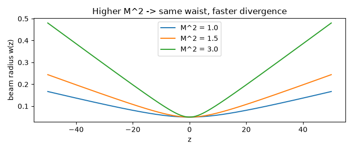
provided the Rayleigh range \(z_R = \pi w_0^2/\lambda\) is rescaled by one dimensionless beam propagation factor \(M^2 \ge 1\) (equal to 1 for an ideal beam, and growing with the severity of multimode content or aberrations). m2_beam_waist() implements this rescaled-Rayleigh-range beam envelope directly, reducing to waist() at \(M^2 = 1\). Below, three beams share the same waist \(w_0 = 0.05\) and wavelength \(\lambda = 0.5\times10^{-3}\) but differ in \(M^2\) (1.0, 1.5, 3.0): the effective Rayleigh range shrinks as \(M^2\) grows, so the same waist diverges increasingly faster away from \(z=0\).

import matplotlib.pyplot as plt
import numpy as np

from physicskit.optics.gaussian import GaussianBeam, m2_beam_waist

Same waist, different beam quality: higher M^2 diverges faster

wavelength, w0 = 0.5e-3, 0.05
z = np.linspace(-50, 50, 400)

fig, ax = plt.subplots(figsize=(7, 3))
for M2 in [1.0, 1.5, 3.0]:
    w = m2_beam_waist(z, wavelength, w0, M2=M2)
    ax.plot(z, w, label=f"M^2 = {M2}")
ax.set_xlabel("z")
ax.set_ylabel("beam radius w(z)")
ax.legend()
ax.set_title("Higher M^2 -> same waist, faster divergence")
fig.tight_layout()

Consistency check: at M^2 = 1, m2_beam_waist must reduce exactly to the ordinary diffraction-limited GaussianBeam.waist – the M^2=1 ideal case Siegman’s formula was built to contain as a special case.

ideal_beam = GaussianBeam(wavelength=wavelength, w0=w0, z0=0.0)
w_ideal = ideal_beam.waist(z)
w_m2_one = m2_beam_waist(z, wavelength, w0, M2=1.0)
print(f"waist w0={w0}, wavelength={wavelength}")
print(f"m2_beam_waist(M2=1.0) matches GaussianBeam.waist(): {np.allclose(w_ideal, w_m2_one)}")

for M2 in [1.0, 1.5, 3.0]:
    w_far = m2_beam_waist(50.0, wavelength, w0, M2=M2)
    print(f"M^2 = {M2}: beam radius at z=50 is {w_far:.4f} ({w_far / w0:.2f}x the waist)")

waist w0=0.05, wavelength=0.0005
m2_beam_waist(M2=1.0) matches GaussianBeam.waist(): True
M^2 = 1.0: beam radius at z=50 is 0.1668 (3.34x the waist)
M^2 = 1.5: beam radius at z=50 is 0.2439 (4.88x the waist)
M^2 = 3.0: beam radius at z=50 is 0.4801 (9.60x the waist)

The full (z, M^2) parameter sweep as one image

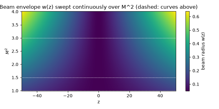
Rather than three discrete M^2 curves, evaluate m2_beam_waist() on a dense 2D grid of both z and M^2 at once: each horizontal slice of the image reproduces one of the curves above, and the image as a whole shows how the beam envelope smoothly degrades as M^2 sweeps continuously from the diffraction-limited case up to strongly multimode beams.

M2_grid = np.linspace(1.0, 4.0, 150)
Z, M2G = np.meshgrid(z, M2_grid)
W = m2_beam_waist(Z, wavelength, w0, M2=M2G)

fig2, ax2 = plt.subplots(figsize=(7, 3.5))
im = ax2.pcolormesh(z, M2_grid, W, shading="auto", cmap="viridis")
fig2.colorbar(im, ax=ax2, label="beam radius w(z)")
for M2 in [1.0, 1.5, 3.0]:
    ax2.axhline(M2, color="w", ls="--", lw=0.6)
ax2.set_xlabel("z")
ax2.set_ylabel(r"$M^2$")
ax2.set_title("Beam envelope w(z) swept continuously over M^2 (dashed: curves above)")
fig2.tight_layout()