Schawlow and Townes: the lasing threshold from the laser rate equations

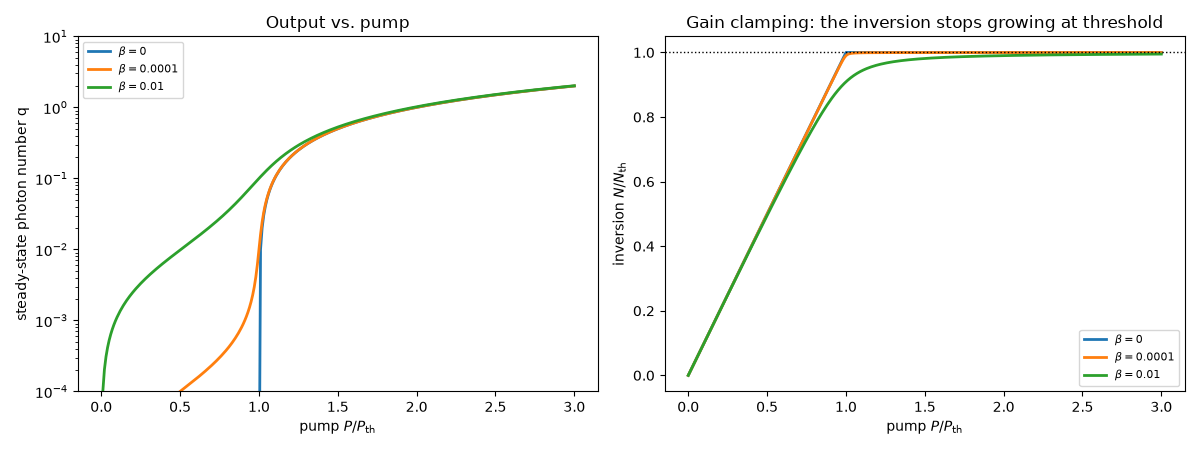
Schawlow and Townes (1958) showed that an optical cavity containing an inverted medium oscillates once the gain from stimulated emission beats the cavity loss. In the rate equations for the inversion \(N\) and the photon number \(q\) (LaserRateEquations) this happens at the threshold inversion \(N_{\rm th} = 1/(B\tau_c)\). 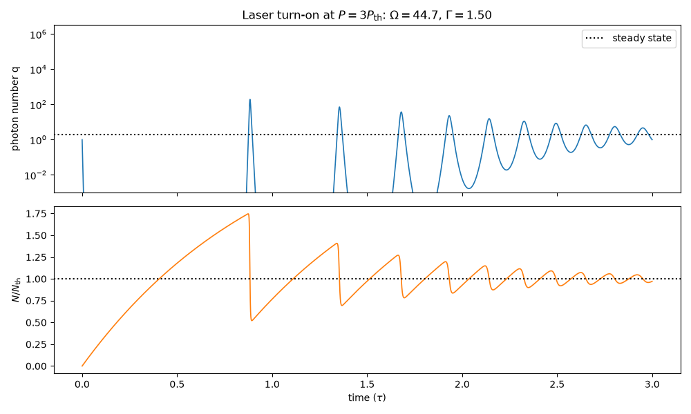Above threshold the inversion is clamped there and the output grows linearly with the pump. When the laser is switched on, it overshoots in a train of spikes that settle through damped relaxation oscillations.

import matplotlib.pyplot as plt
import numpy as np
from scipy.signal import find_peaks

from physicskit.optics.lasers import LaserRateEquations

tau, tau_c, B = 1.0, 1e-3, 1.0
P_th = LaserRateEquations(tau=tau, tau_c=tau_c, B=B).threshold_pump

Threshold and gain clamping

A small spontaneous-emission fraction \(\beta\) into the lasing mode rounds the threshold; with \(\beta \to 0\) it becomes a sharp kink.

r = np.linspace(0, 3, 301)
fig, axes = plt.subplots(1, 2, figsize=(12, 4.5))
for beta in (0.0, 1e-4, 1e-2):
    ss = np.array([LaserRateEquations(pump=x * P_th, tau=tau, tau_c=tau_c, B=B, beta=beta).steady_state() for x in r])
    axes[0].semilogy(r, np.maximum(ss[:, 1], 1e-6), lw=2, label=rf"$\beta = {beta:g}$")
    axes[1].plot(r, ss[:, 0] * B * tau_c, lw=2, label=rf"$\beta = {beta:g}$")
axes[0].set_xlabel(r"pump $P / P_{\rm th}$")
axes[0].set_ylabel("steady-state photon number q")
axes[0].set_ylim(1e-4, 1e1)
axes[0].set_title("Output vs. pump")
axes[0].legend(fontsize=8)
axes[1].axhline(1, color="k", ls=":", lw=1)
axes[1].set_xlabel(r"pump $P / P_{\rm th}$")
axes[1].set_ylabel(r"inversion $N / N_{\rm th}$")
axes[1].set_title("Gain clamping: the inversion stops growing at threshold")
axes[1].legend(fontsize=8)
fig.tight_layout()

Turn-on: spiking and relaxation oscillations

Switching the pump on at \(P = 3P_{\rm th}\), the inversion overshoots the threshold before the photon number, seeded by a single photon, catches up. The system then relaxes to the steady state with frequency \(\Omega\) and damping \(\Gamma\) from relaxation_oscillation().

laser = LaserRateEquations(pump=3 * P_th, tau=tau, tau_c=tau_c, B=B)
t, N, q = laser.integrate(t_max=3.0, dt=2e-5, N0=0.0, q0=1.0)
N_s, q_s = laser.steady_state()
Omega, Gamma = laser.relaxation_oscillation()

fig2, ax2 = plt.subplots(2, 1, figsize=(10, 6), sharex=True)
ax2[0].plot(t, q, lw=1.2)
ax2[0].axhline(q_s, color="k", ls=":", label="steady state")
ax2[0].set_ylabel("photon number q")
ax2[0].set_yscale("log")
ax2[0].set_ylim(1e-3, None)
ax2[0].set_title(rf"Laser turn-on at $P = 3P_{{\rm th}}$: $\Omega = {Omega:.1f}$, $\Gamma = {Gamma:.2f}$")
ax2[0].legend()
ax2[1].plot(t, N / laser.threshold_inversion, lw=1.2, color="C1")
ax2[1].axhline(1, color="k", ls=":")
ax2[1].set_ylabel(r"$N / N_{\rm th}$")
ax2[1].set_xlabel(r"time ($\tau$)")
fig2.tight_layout()

print(f"threshold pump P_th = {P_th:g}, steady state (N, q) = ({N_s:g}, {q_s:g})")
print(f"relaxation oscillation period 2pi/Omega = {2 * np.pi / Omega:.4f}")

threshold pump P_th = 1000, steady state (N, q) = (1000, 2)
relaxation oscillation period 2pi/Omega = 0.1406

Check

Above threshold the inversion clamps at N_th and q = (P - P_th) tau_c; relaxation oscillations e^(-Gamma t) cos(Omega t) with Gamma = r / 2 tau, Omega = sqrt((r - 1) / (tau tau_c) - Gamma^2), r = P / P_th – the (nonlinear) turn-on spikes come ever closer until, near steady state, they are spaced 2 pi / Omega – and their heights decay toward the steady state.

assert abs(N_s - laser.threshold_inversion) < 1e-9 and abs(q_s - 2 * P_th * tau_c) < 1e-9
for x in (1.5, 2.0, 3.0):
    N_x, _ = LaserRateEquations(pump=x * P_th, tau=tau, tau_c=tau_c, B=B).steady_state()
    assert abs(N_x / laser.threshold_inversion - 1) < 1e-9
assert abs(Gamma - 3 / (2 * tau)) < 1e-12 and abs(Omega - np.sqrt(2 / (tau * tau_c) - Gamma**2)) < 1e-9 * Omega
spikes, _ = find_peaks(q, prominence=0.01 * q.max())
late = spikes[t[spikes] > 2.5]
assert len(late) >= 3 and abs(np.diff(t[late]).mean() / (2 * np.pi / Omega) - 1) < 0.1
assert np.all(np.diff(q[spikes]) < 0) and q[spikes[-1]] < 0.2 * q[spikes[0]]