Haken’s laser-Lorenz analogy: Maxwell-Bloch dynamics and laser chaos

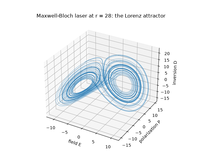
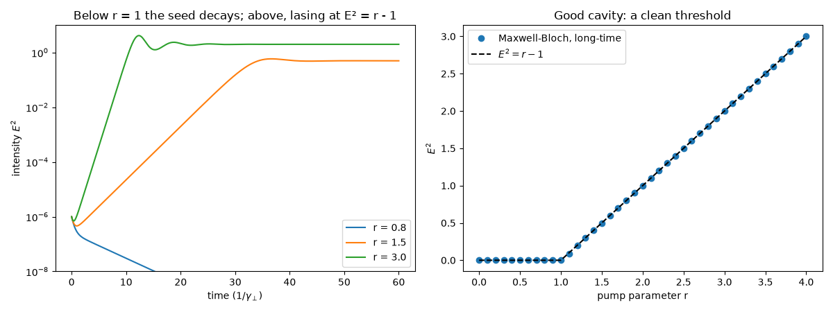
Rate equations ignore the atomic polarization. Keeping it, the semiclassical single-mode laser obeys the Maxwell-Bloch equations for the field \(E\), polarization \(P\) and inversion \(D\) (MaxwellBloch). Haken (1975) noticed these are the Lorenz equations. The laser switches on at \(r = 1\), and in a “bad cavity” (\(\kappa > \gamma_\perp + \gamma_\parallel\)) the steady lasing state becomes unstable at a second threshold \(r_H\), after which the output intensity is chaotic.

import matplotlib.pyplot as plt
import numpy as np

from physicskit.optics.lasers import MaxwellBloch

First threshold: the laser switches on

fig, axes = plt.subplots(1, 2, figsize=(12, 4.5))
for r in (0.8, 1.5, 3.0):
    mb = MaxwellBloch(kappa=1.0, gamma_perp=1.0, gamma_par=0.5, r=r)
    t, y = mb.integrate([1e-3, 0.0, r], t_max=60.0, dt=0.01)
    axes[0].semilogy(t, y[:, 0] ** 2 + 1e-12, lw=1.5, label=f"r = {r}")
axes[0].set_xlabel(r"time ($1/\gamma_\perp$)")
axes[0].set_ylabel(r"intensity $E^2$")
axes[0].set_ylim(1e-8, 10)
axes[0].set_title("Below r = 1 the seed decays; above, lasing at E² = r - 1")
axes[0].legend()

r_grid = np.linspace(0, 4, 41)
I_final = []
for r in r_grid:
    _, y = MaxwellBloch(kappa=1.0, gamma_perp=1.0, gamma_par=0.5, r=r).integrate([1e-3, 0.0, r], t_max=150.0, dt=0.02)
    I_final.append(y[-1, 0] ** 2)
axes[1].plot(r_grid, I_final, "o", label="Maxwell-Bloch, long-time")
axes[1].plot(r_grid, np.maximum(r_grid - 1, 0), "k--", label=r"$E^2 = r - 1$")
axes[1].set_xlabel("pump parameter r")
axes[1].set_ylabel(r"$E^2$")
axes[1].set_title("Good cavity: a clean threshold")
axes[1].legend()
fig.tight_layout()

Second threshold: chaotic output in a bad cavity

With \(\sigma = \kappa/\gamma_\perp = 10\) and \(b = \gamma_\parallel/\gamma_\perp = 8/3\), Lorenz’s own parameters, the lasing state loses stability at \(r_H \approx 24.74\).

mb = MaxwellBloch(kappa=10.0, gamma_perp=1.0, gamma_par=8 / 3)
print(f"second (Haken) threshold r_H = {mb.second_threshold:.4f}")
fig2, axes2 = plt.subplots(2, 1, figsize=(10, 6), sharex=True)
for ax, r in zip(axes2, (20.0, 28.0)):
    mb.r = r
    t, y = mb.integrate([1.0, 1.0, 1.0], t_max=40.0, dt=0.002)
    ax.plot(t, y[:, 0], lw=0.8)
    ax.axhline(np.sqrt(r - 1), color="k", ls=":", lw=1)
    ax.axhline(-np.sqrt(r - 1), color="k", ls=":", lw=1)
    ax.set_ylabel("field E")
    state = "stable lasing" if r < mb.second_threshold else "chaos"
    ax.set_title(f"r = {r} ({state}; $r_H$ = {mb.second_threshold:.2f})")
axes2[-1].set_xlabel(r"time ($1/\gamma_\perp$)")
fig2.tight_layout()

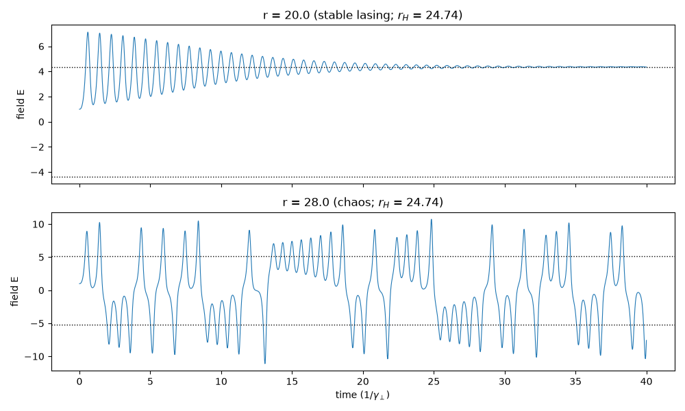
second (Haken) threshold r_H = 24.7368

The strange attractor in (E, P, D) space

mb.r = 28.0
_, y = mb.integrate([1.0, 1.0, 1.0], t_max=60.0, dt=0.002)
y = y[5000:]
fig3 = plt.figure(figsize=(6.5, 5.5))
ax3 = fig3.add_subplot(projection="3d")
ax3.plot(y[:, 0], y[:, 1], y[:, 2], lw=0.4)
ax3.set_xlabel("field E")
ax3.set_ylabel("polarization P")
ax3.set_zlabel("inversion D")
ax3.set_title("Maxwell-Bloch laser at r = 28: the Lorenz attractor")

Text(0.5, 1.0, 'Maxwell-Bloch laser at r = 28: the Lorenz attractor')

Check

Good cavity: lasing threshold at r = 1 with E^2 = r - 1 above it; bad cavity: Haken’s second threshold r_H = sigma (sigma + b + 3) / (sigma - b - 1).

np.testing.assert_allclose(I_final, np.maximum(r_grid - 1, 0), atol=0.02)
sigma_l, b_l = 10.0, 8 / 3
assert abs(mb.second_threshold - sigma_l * (sigma_l + b_l + 3) / (sigma_l - b_l - 1)) < 1e-9