Glauber’s coherent states: displaced vacuum, Poissonian statistics

Roy Glauber identified the coherent states \(|\alpha\rangle\) – eigenstates of the annihilation operator, \(\hat a|\alpha\rangle = \alpha|\alpha\rangle\) – as the quantum states that most closely reproduce a classical, stable-amplitude light wave: a positive Gaussian in phase space, displaced away from the origin, whose photon number follows a Poissonian distribution – the quantum-mechanical signature of what an ideal, shot-noise-limited laser beam actually is. coherent_state() constructs this state directly in a truncated Fock basis (dimension cutoff),

\[\lvert\alpha\rangle = e^{-\lvert\alpha\rvert^2/2} \sum_{n=0}^{\infty} \frac{\alpha^n}{\sqrt{n!}}\,\lvert n\rangle,\]

for use with compute_wigner_function() and any of the package’s other state-based quantum-optics tools. Below, \(\alpha = 2+i\) (mean photon number \(\langle n\rangle = |\alpha|^2 = 5\)) is used to compute both the phase-space Wigner function \(W(x,p)\) and the photon-number distribution \(P(n) = |\langle n|\alpha\rangle|^2\).

import matplotlib.pyplot as plt
import numpy as np

from physicskit.optics.quantum_optics import coherent_state, compute_wigner_function

A coherent state \(|\alpha\rangle\), its phase-space blob and photon statistics

cutoff = 30
alpha = 2.0 + 1.0j
psi = coherent_state(alpha, cutoff)

n = np.arange(cutoff)
P_n = np.abs(psi) ** 2
mean_n = np.sum(n * P_n)
var_n = np.sum(n**2 * P_n) - mean_n**2

x = np.linspace(-6, 6, 121)
p = np.linspace(-6, 6, 121)
W = compute_wigner_function(psi, x, p)

A coherent state’s Wigner function is a Gaussian bump displaced from the origin (never negative), and its photon-number distribution is Poissonian: mean and variance both equal \(|\alpha|^2\).

fig, axes = plt.subplots(1, 2, figsize=(9, 4))
axes[0].contourf(x, p, W.T, levels=40, cmap="RdBu_r")
axes[0].set_title(r"$W(x,p)$ for a displaced coherent state")
axes[0].set_xlabel("x")
axes[0].set_ylabel("p")
axes[1].bar(n, P_n)
axes[1].axvline(mean_n, color="r", ls="--", label=r"$\langle n\rangle=|\alpha|^2$")
axes[1].set_title("Poissonian photon-number distribution")
axes[1].set_xlabel("n")
axes[1].legend()
fig.tight_layout()

print(f"alpha = {alpha}, |alpha|^2 = {abs(alpha) ** 2:.4f}")
print(f"measured <n> = {mean_n:.4f}   measured Var(n) = {var_n:.4f}")
print("Poissonian statistics: <n> = Var(n) = |alpha|^2, confirmed above.")
print(f"minimum of W(x,p) over the grid: {W.min():.6f} (non-negative: classical state)")

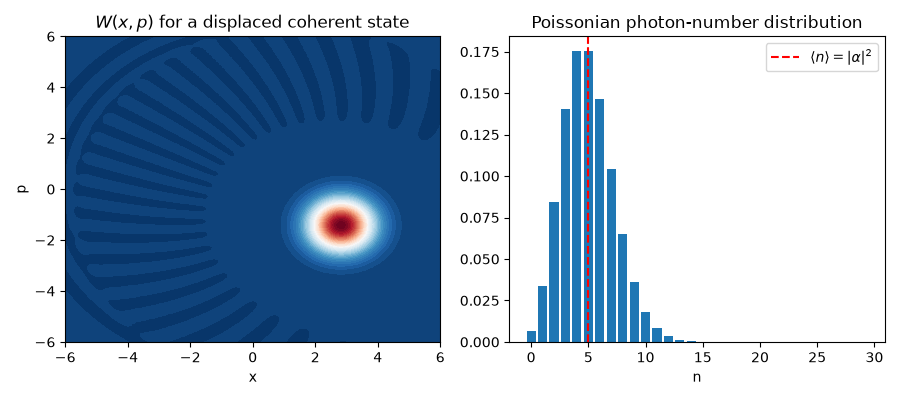
alpha = (2+1j), |alpha|^2 = 5.0000
measured <n> = 5.0000   measured Var(n) = 5.0000
Poissonian statistics: <n> = Var(n) = |alpha|^2, confirmed above.
minimum of W(x,p) over the grid: -0.000000 (non-negative: classical state)