Einstein’s light quanta and the photoelectric effect

Einstein (1905) proposed that light of frequency \(\nu\) is absorbed in quanta of energy \(h\nu\). One quantum ejects one electron, which leaves the metal with at most

\[K_{\max} = h\nu - W,\]

where \(W\) is the metal’s work function. A classical wave predicts none of what follows from this: no emission below the threshold \(\nu_0 = W/h\) however bright the light, electron energies set by the colour rather than the brightness, and a straight line of stopping voltage against frequency with the universal slope \(h/e\). Millikan (1916) measured that line and got Planck’s constant from it. This example reproduces the three signatures with values from physicskit.constants, then counts photons in a faint beam.

import matplotlib.pyplot as plt
import numpy as np

from physicskit.constants import ELEMENTARY_CHARGE, C, H

EV = ELEMENTARY_CHARGE
metals = {"caesium": 2.14, "sodium": 2.36, "zinc": 4.33}  # work functions [eV]

Threshold and slope

\(eV_{\rm stop} = h\nu - W\): one line per metal, all with the same slope, each cut off at its own threshold frequency.

nu = np.linspace(3e14, 1.6e15, 400)
fig1, ax1 = plt.subplots(figsize=(6, 4))
for (name, W), color in zip(metals.items(), ["goldenrod", "steelblue", "firebrick"]):
    K = H * nu / EV - W
    ax1.plot(nu / 1e15, np.where(K > 0, K, np.nan), color=color, label=f"{name}, W = {W} eV")
    nu0 = W * EV / H
    ax1.plot(nu0 / 1e15, 0, "o", color=color)
    print(f"{name:8s}: threshold nu0 = {nu0 / 1e15:.3f} PHz  (wavelength {C / nu0 * 1e9:.0f} nm)")
ax1.set_xlabel(r"frequency $\nu$ [PHz]")
ax1.set_ylabel(r"$K_{\max}$ = e V$_{stop}$ [eV]")
ax1.set_title(r"$K_{\max} = h\nu - W$: same slope, different thresholds")
ax1.legend(fontsize=8)
fig1.tight_layout()

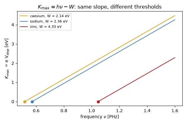
caesium : threshold nu0 = 0.517 PHz  (wavelength 579 nm)
sodium  : threshold nu0 = 0.571 PHz  (wavelength 525 nm)
zinc    : threshold nu0 = 1.047 PHz  (wavelength 286 nm)

Millikan’s measurement of \(h\)

Stopping voltages for sodium at seven mercury-lamp lines, with 20 mV of measurement noise. The fitted slope is \(h/e\); the intercept is the work function.

rng = np.random.default_rng(1916)
lines_nm = np.array([253.7, 296.7, 312.6, 334.1, 365.0, 404.7, 435.8])
nu_lines = C / (lines_nm * 1e-9)
V_stop = H * nu_lines / EV - metals["sodium"] + rng.normal(0, 0.02, lines_nm.size)
slope, intercept = np.polyfit(nu_lines, V_stop, 1)
print(f"\nfitted h = {slope * EV:.4e} J s   (CODATA {H:.4e})")
print(f"fitted W = {-intercept:.3f} eV   (input {metals['sodium']} eV)")

fitted h = 6.6400e-34 J s   (CODATA 6.6261e-34)
fitted W = 2.353 eV   (input 2.36 eV)

Brightness changes the current, not the energy

At 400 nm on sodium, doubling the intensity doubles the photon flux and hence the photocurrent (quantum efficiency 10%), while every electron still leaves with the same \(K_{\max}\). Below threshold, at 600 nm, nothing is emitted at any intensity.

area = 1e-4  # m^2
for wavelength_nm in (400.0, 600.0):
    E_photon = H * C / (wavelength_nm * 1e-9)
    K = E_photon / EV - metals["sodium"]
    for intensity in (1.0, 2.0, 4.0):  # W/m^2
        flux = intensity * area / E_photon
        current = 0.1 * flux * EV if K > 0 else 0.0
        print(f"{wavelength_nm:.0f} nm, {intensity:.0f} W/m^2: photocurrent {current * 1e6:6.2f} uA, K_max = {max(K, 0):.2f} eV")

400 nm, 1 W/m^2: photocurrent   3.23 uA, K_max = 0.74 eV
400 nm, 2 W/m^2: photocurrent   6.45 uA, K_max = 0.74 eV
400 nm, 4 W/m^2: photocurrent  12.90 uA, K_max = 0.74 eV
600 nm, 1 W/m^2: photocurrent   0.00 uA, K_max = 0.00 eV
600 nm, 2 W/m^2: photocurrent   0.00 uA, K_max = 0.00 eV
600 nm, 4 W/m^2: photocurrent   0.00 uA, K_max = 0.00 eV

Light arrives in lumps

A 1 fW beam at 500 nm carries about 2500 photons per second. Each absorbed quantum is a separate detector click at a random moment, so counts in equal time bins scatter with Poisson statistics, and the clicks don’t smear out into a smooth classical intensity.

P, wavelength = 1e-15, 500e-9
rate = P / (H * C / wavelength)
t_clicks = np.cumsum(rng.exponential(1 / rate, size=int(rate * 1.5)))
t_clicks = t_clicks[t_clicks < 1.0]
counts, _ = np.histogram(t_clicks, bins=100, range=(0, 1.0))
print(f"\nphoton rate {rate:.0f} /s; counts per 10 ms bin: mean {counts.mean():.1f}, variance {counts.var():.1f}")

fig2, (ax2, ax3) = plt.subplots(1, 2, figsize=(11, 3.6))
ax2.plot(nu_lines / 1e15, V_stop, "o", color="steelblue", label="stopping voltage")
ax2.plot(nu_lines / 1e15, np.polyval([slope, intercept], nu_lines), "--", color="orange", label=f"slope h/e -> h = {slope * EV:.3e}")
ax2.set_xlabel(r"$\nu$ [PHz]")
ax2.set_ylabel(r"$V_{stop}$ [V]")
ax2.set_title("Millikan: Planck's constant from a straight line")
ax2.legend(fontsize=8)
ax3.eventplot(t_clicks[t_clicks < 0.02] * 1e3, color="k", linelengths=0.8)
ax3.set_xlabel("time [ms]")
ax3.set_yticks([])
ax3.set_title("1 fW of green light: individual quanta")
fig2.tight_layout()

plt.show()

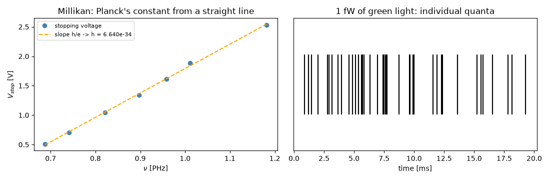
photon rate 2517 /s; counts per 10 ms bin: mean 25.8, variance 24.0

Check

K_max = h nu - W: the stopping-voltage slope gives h and the intercept W; no photocurrent below threshold at any intensity; photon counts are Poissonian (variance ~ mean).

assert abs(slope * EV / H - 1) < 0.01 and abs(-intercept - metals["sodium"]) < 0.03
assert H * C / 600e-9 / EV < metals["sodium"] < H * C / 400e-9 / EV
assert abs(counts.var() / counts.mean() - 1) < 0.3