Tomonaga, Schwinger, Feynman, and Dyson: renormalized QED

Renormalized QED’s cleanest tree-level prediction is \(e^+e^-\to\mu^+\mu^-\), whose differential cross section in the massless-fermion limit is

\[\frac{d\sigma}{d\Omega} = \frac{\alpha^2}{4s}\left(1+\cos^2\theta\right),\]

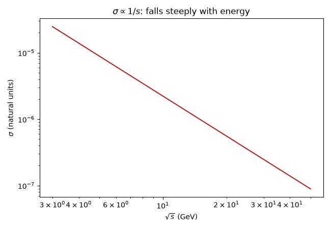
confirmed to good precision once electron-positron colliders reached sufficient energy, and used ever since to calibrate new machines’ luminosity. This example plots qed_dsigma_domega_mumu()’s \(1+\cos^2\theta\) angular shape, checks the total cross section qed_total_cross_section_mumu() against direct numerical integration of the differential form, and shows how the cross section falls as \(1/s\) with increasing center-of-mass energy.

import matplotlib.pyplot as plt
import numpy as np

from physicskit.particle.electroweak import qed_dsigma_domega_mumu, qed_total_cross_section_mumu
from physicskit.particle.visualizers import animate_qed_angular_distribution

The angular shape: forward-backward symmetric, peaked at the poles

sqrt_s = 10.0  # GeV
theta = np.linspace(0.0, np.pi, 300)
dsigma = qed_dsigma_domega_mumu(np.cos(theta), sqrt_s)

fig1, ax1 = plt.subplots(figsize=(6, 4.8), subplot_kw={"projection": "polar"})
ax1.plot(theta, dsigma, color="steelblue")
ax1.plot(-theta, dsigma, color="steelblue")  # mirror for the full 2D shape
ax1.set_title(rf"$d\sigma/d\Omega \propto 1+\cos^2\theta$ at $\sqrt{{s}}$={sqrt_s} GeV")
fig1.tight_layout()

print(f"forward (theta=0): {qed_dsigma_domega_mumu(1.0, sqrt_s):.6e}")
print(f"transverse (theta=90 deg): {qed_dsigma_domega_mumu(0.0, sqrt_s):.6e}")
ratio_fwd_transverse = qed_dsigma_domega_mumu(1.0, sqrt_s) / qed_dsigma_domega_mumu(0.0, sqrt_s)
print(f"ratio forward/transverse: {ratio_fwd_transverse:.4f} (should be exactly 2.0, from 1+cos^2(0)=2 vs 1+cos^2(90deg)=1)")

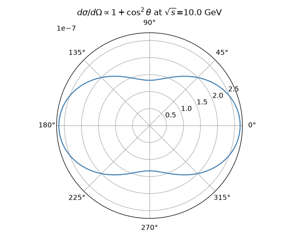
forward (theta=0): 2.662568e-07
transverse (theta=90 deg): 1.331284e-07
ratio forward/transverse: 2.0000 (should be exactly 2.0, from 1+cos^2(0)=2 vs 1+cos^2(90deg)=1)

Checking the total cross section by direct integration

cos_theta_fine = np.linspace(-1.0, 1.0, 200001)
dsigma_fine = qed_dsigma_domega_mumu(cos_theta_fine, sqrt_s)
# integrate over the full solid angle: dOmega = dphi * d(cos theta), phi in [0, 2pi]
sigma_numeric = 2.0 * np.pi * np.trapezoid(dsigma_fine, cos_theta_fine)
sigma_formula = qed_total_cross_section_mumu(sqrt_s)
print(f"\ntotal cross section, numerical integration: {sigma_numeric:.8e}")
print(f"total cross section, closed-form 4*pi*alpha^2/(3s): {sigma_formula:.8e}")
print(f"relative difference: {abs(sigma_numeric - sigma_formula) / sigma_formula:.2e}")

total cross section, numerical integration: 2.23058752e-06
total cross section, closed-form 4*pi*alpha^2/(3s): 2.23058752e-06
relative difference: 1.25e-11

Falling as 1/s with center-of-mass energy

sqrt_s_values = np.linspace(3.0, 50.0, 200)
sigma_values = np.array([qed_total_cross_section_mumu(s) for s in sqrt_s_values])

fig2, ax2 = plt.subplots(figsize=(6.5, 4.5))
ax2.loglog(sqrt_s_values, sigma_values, color="firebrick")
ax2.set_xlabel(r"$\sqrt{s}$ (GeV)")
ax2.set_ylabel(r"$\sigma$ (natural units)")
ax2.set_title(r"$\sigma \propto 1/s$: falls steeply with energy")
fig2.tight_layout()

The angular shape’s overall normalization, swept across sqrt(s)

anim = animate_qed_angular_distribution(np.linspace(5.0, 30.0, 20))

plt.show()