Higgs, Brout-Englert, and Guralnik-Hagen-Kibble: symmetry breaking

In 1964, three independent groups showed how a gauge symmetry can be spontaneously broken while still keeping the theory’s equations exactly symmetric – the mechanism that gives the \(W\) and \(Z\) bosons their mass while leaving the photon massless. The classical, single-field toy version is a real scalar in the double-well potential \(V(\phi)=-a\phi^2+b\phi^4\): the field must “choose” one of two degenerate minima \(\phi=\pm v\), \(v=\sqrt{a/(2b)}\). This example evolves higgs_field_rollover() from a tiny perturbation near the unstable symmetric point, watches it settle into one of the two vacua, and shows that a mirrored initial perturbation settles into the other, degenerate vacuum – spontaneous symmetry breaking captured directly.

import matplotlib.pyplot as plt
import numpy as np

from physicskit.particle.electroweak import higgs_field_rollover, higgs_potential, higgs_vev
from physicskit.particle.visualizers import animate_higgs_rollover

The double-well potential and its vacuum expectation value

a, b = 1.0, 1.0
v = higgs_vev(a, b)
print(f"potential parameters: a={a}, b={b}")
print(f"vacuum expectation value v = sqrt(a/2b) = {v:.6f}")
print(f"V(0) = {higgs_potential(0.0, a, b):.6f} (unstable symmetric point)")
print(f"V(+v) = {higgs_potential(v, a, b):.6f}, V(-v) = {higgs_potential(-v, a, b):.6f} (degenerate true minima)")

potential parameters: a=1.0, b=1.0
vacuum expectation value v = sqrt(a/2b) = 0.707107
V(0) = 0.000000 (unstable symmetric point)
V(+v) = -0.250000, V(-v) = -0.250000 (degenerate true minima)

A tiny perturbation decides which vacuum the field falls into

t = np.linspace(0.0, 60.0, 800)
phi_plus, _ = higgs_field_rollover(1e-3, 0.0, a, b, t, damping=0.08)
phi_minus, _ = higgs_field_rollover(-1e-3, 0.0, a, b, t, damping=0.08)

print(f"\nstarting at phi0=+1e-3: field settles at phi={phi_plus[-1]:.6f} (target +v={v:.6f})")
print(f"starting at phi0=-1e-3: field settles at phi={phi_minus[-1]:.6f} (target -v={-v:.6f})")
print("(an infinitesimally different initial nudge -- the only difference between the two runs --")
print(" decides which of the two physically identical vacua the field ends up in)")

fig1, (ax1, ax2) = plt.subplots(1, 2, figsize=(11, 4.5))
phi_range = np.linspace(-1.3 * v, 1.3 * v, 400)
ax1.plot(phi_range, higgs_potential(phi_range, a, b), color="gray")
ax1.plot(v, higgs_potential(v, a, b), "o", color="steelblue", ms=8)
ax1.plot(-v, higgs_potential(-v, a, b), "o", color="firebrick", ms=8)
ax1.plot(0, 0, "o", color="0.3", ms=6)
ax1.set_xlabel(r"$\phi$")
ax1.set_ylabel(r"$V(\phi)$")
ax1.set_title("The Mexican-hat / double-well potential")

ax2.plot(t, phi_plus, color="steelblue", label=r"$\phi_0=+10^{-3}$")
ax2.plot(t, phi_minus, color="firebrick", label=r"$\phi_0=-10^{-3}$")
ax2.axhline(v, color="0.6", ls="--", lw=1)
ax2.axhline(-v, color="0.6", ls="--", lw=1)
ax2.set_xlabel("t")
ax2.set_ylabel(r"$\phi(t)$")
ax2.set_title("Spontaneous symmetry breaking: which vacuum, decided by an infinitesimal nudge")
ax2.legend(fontsize=8)
fig1.tight_layout()

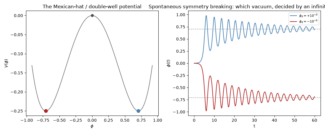
starting at phi0=+1e-3: field settles at phi=0.685442 (target +v=0.707107)
starting at phi0=-1e-3: field settles at phi=-0.685442 (target -v=-0.707107)
(an infinitesimally different initial nudge -- the only difference between the two runs --
 decides which of the two physically identical vacua the field ends up in)

The rollover, animated

anim = animate_higgs_rollover(phi_plus, a, b)

plt.show()