Glashow, Weinberg, and Salam: electroweak unification

Glashow (1961), Weinberg (1967), and Salam (1968) showed that the electromagnetic and weak interactions are two faces of a single \(SU(2)\times U(1)\) gauge theory, spontaneously broken by the Higgs mechanism into the massless photon (electromagnetism) and the massive \(W^\pm,Z^0\) bosons (the weak force). One mixing angle \(\theta_W\) ties the two together. With the fine-structure constant and Fermi’s constant it predicts the boson masses,

\[M_W = \left(\frac{\pi\alpha}{\sqrt2\,G_F}\right)^{1/2}\frac{1}{\sin\theta_W}, \qquad M_Z = \frac{M_W}{\cos\theta_W}.\]

This example puts the theory’s pieces side by side: qed_total_cross_section_mumu(), the electromagnetic sector at low energy; higgs_vev(), the symmetry-breaking scale; and the tree-level \(W\) and \(Z\) mass predictions as a function of \(\sin^2\theta_W\).

import matplotlib.pyplot as plt
import numpy as np

from physicskit.particle.electroweak import higgs_potential, higgs_vev, qed_total_cross_section_mumu

Piece 1: the electromagnetic sector, reproduced at low energy

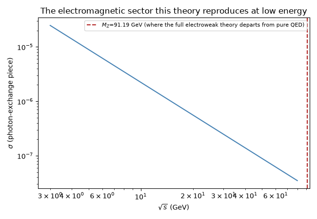
Below the Z pole (sqrt(s) << M_Z ~ 91 GeV), the electroweak theory’s prediction for e+e- -> mu+mu- reduces to pure photon exchange – the same QED cross section already checked on its own terms in the renormalized-QED example.

sqrt_s_values = np.linspace(3.0, 80.0, 200)
sigma_qed = np.array([qed_total_cross_section_mumu(s) for s in sqrt_s_values])
M_Z = 91.19  # GeV, for reference -- not itself predicted by the pieces modeled here

fig1, ax1 = plt.subplots(figsize=(6.5, 4.5))
ax1.loglog(sqrt_s_values, sigma_qed, color="steelblue")
ax1.axvline(M_Z, color="firebrick", ls="--", label=f"$M_Z$={M_Z} GeV (where the full electroweak theory departs from pure QED)")
ax1.set_xlabel(r"$\sqrt{s}$ (GeV)")
ax1.set_ylabel(r"$\sigma$ (photon-exchange piece)")
ax1.set_title("The electromagnetic sector this theory reproduces at low energy")
ax1.legend(fontsize=8)
fig1.tight_layout()

Piece 2: the symmetry-breaking scale setting the W/Z masses

The same spontaneous-symmetry-breaking mechanism modeled in the Higgs example gives the W and Z bosons their mass (schematically, M_W, M_Z ~ g*v for the theory’s gauge couplings g) while leaving the photon exactly massless – a direct structural consequence of which combination of the SU(2)xU(1) generators remains unbroken.

a, b = 1.0, 1.0
v = higgs_vev(a, b)
print(f"symmetry-breaking scale v = {v:.6f} (schematic units)")
print("the W and Z acquire mass proportional to this scale (times the theory's gauge couplings);")
print("the photon corresponds to the one gauge direction left exactly unbroken -- massless by construction.")

phi_range = np.linspace(-1.3 * v, 1.3 * v, 400)
fig2, ax2 = plt.subplots(figsize=(6, 4.5))
ax2.plot(phi_range, higgs_potential(phi_range, a, b), color="gray")
ax2.plot([v, -v], [higgs_potential(v, a, b), higgs_potential(-v, a, b)], "o", color="firebrick", ms=8)
ax2.set_xlabel(r"$\phi$")
ax2.set_ylabel(r"$V(\phi)$")
ax2.set_title("The symmetry-breaking scale that sets M_W, M_Z (schematic)")
fig2.tight_layout()

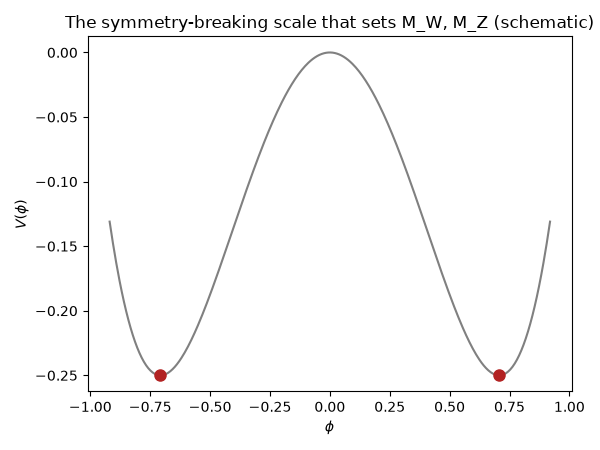
symmetry-breaking scale v = 0.707107 (schematic units)
the W and Z acquire mass proportional to this scale (times the theory's gauge couplings);
the photon corresponds to the one gauge direction left exactly unbroken -- massless by construction.

Piece 3: the W and Z masses from the mixing angle

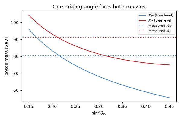
Tree level, using the low-energy alpha = 1/137 and G_F. Values of sin^2 theta_W between 0.2 and 0.25 put M_W near 75-83 GeV and M_Z near 85-93 GeV, out of reach of any 1970s accelerator; UA1 and UA2 found them in 1983 at 81 and 93 GeV (loop corrections, mainly the running of alpha, account for the few-GeV difference from this estimate).

alpha, G_F = 1 / 137.036, 1.1663787e-5  # GeV^-2
A0 = np.sqrt(np.pi * alpha / (np.sqrt(2) * G_F))
s2 = np.linspace(0.15, 0.45, 200)
M_W = A0 / np.sqrt(s2)
M_Z = M_W / np.sqrt(1 - s2)
s2_ref = 0.23
print(f"\n(pi alpha / sqrt2 G_F)^1/2 = {A0:.2f} GeV")
print(f"sin^2 theta_W = {s2_ref}: M_W = {A0 / np.sqrt(s2_ref):.1f} GeV, M_Z = {A0 / np.sqrt(s2_ref * (1 - s2_ref)):.1f} GeV")

fig3, ax3 = plt.subplots(figsize=(6, 4))
ax3.plot(s2, M_W, color="steelblue", label=r"$M_W$ (tree level)")
ax3.plot(s2, M_Z, color="firebrick", label=r"$M_Z$ (tree level)")
ax3.axhline(80.4, color="steelblue", ls=":", label="measured $M_W$")
ax3.axhline(91.19, color="firebrick", ls=":", label="measured $M_Z$")
ax3.set_xlabel(r"$\sin^2\theta_W$")
ax3.set_ylabel("boson mass [GeV]")
ax3.set_title("One mixing angle fixes both masses")
ax3.legend(fontsize=8)
fig3.tight_layout()

plt.show()

(pi alpha / sqrt2 G_F)^1/2 = 37.28 GeV
sin^2 theta_W = 0.23: M_W = 77.7 GeV, M_Z = 88.6 GeV

Check

Tree level: M_W = (pi alpha / sqrt(2) G_F)^(1/2) / sin(theta_W), M_Z = M_W / cos(theta_W).

assert abs(A0 - 37.28) < 0.01
np.testing.assert_allclose(M_W / M_Z, np.sqrt(1 - s2), rtol=1e-12)
assert abs(A0 / np.sqrt(0.23) - 77.7) < 0.1