Gargamelle: the discovery of weak neutral currents

Every weak process seen before 1973 changed the charge of the particles involved: a neutrino came in, a charged muon or electron came out (charged current, \(W^\pm\) exchange). The electroweak theory also required a neutral current, \(Z^0\) exchange, where the neutrino scatters and leaves as a neutrino. In 1973 the Gargamelle bubble chamber at CERN found both kinds of evidence in its neutrino and antineutrino beams: hadron showers with no outgoing muon, and a single electron knocked forward by an invisible neutrino.

The neutral-current rate depends on the weak mixing angle. For deep-inelastic scattering on an isoscalar target, Llewellyn Smith’s quark-model ratios are

\[R_\nu = \frac{\sigma_{NC}}{\sigma_{CC}}(\nu) = \tfrac12 - \sin^2\theta_W + \tfrac59\sin^4\theta_W\,(1+r), \qquad R_{\bar\nu} = \tfrac12 - \sin^2\theta_W + \tfrac59\sin^4\theta_W\,(1+1/r),\]

with \(r=\sigma_{CC}(\bar\nu)/\sigma_{CC}(\nu)\approx0.37\). This example fits Gargamelle’s measured ratios for \(\sin^2\theta_W\), simulates the event counting behind them, and computes the \(\nu_\mu e\to\nu_\mu e\) rate that the single-electron event tested.

import matplotlib.pyplot as plt
import numpy as np

r_cc = 0.37
R_nu_obs, R_nu_err = 0.21, 0.03
R_nubar_obs, R_nubar_err = 0.45, 0.09


def R_nu(s2):
    return 0.5 - s2 + 5 / 9 * s2**2 * (1 + r_cc)


def R_nubar(s2):
    return 0.5 - s2 + 5 / 9 * s2**2 * (1 + 1 / r_cc)

Counting events without a muon

A neutral-current event has a hadron shower and no muon track. Simulate a neutrino exposure at \(\sin^2\theta_W=0.38\), close to what Gargamelle’s data preferred, with a 10% chance of a charged-current muon escaping unseen (a background the experiment had to subtract).

rng = np.random.default_rng(1973)
s2_true, n_events, p_missed = 0.38, 1500, 0.10
is_nc = rng.uniform(size=n_events) < R_nu(s2_true) / (1 + R_nu(s2_true))
muonless = is_nc | (~is_nc & (rng.uniform(size=n_events) < p_missed))
n_muonless, n_muon = muonless.sum(), (~muonless).sum()
R_raw = n_muonless / n_muon
R_corr = (n_muonless - p_missed * n_muon / (1 - p_missed)) / (n_muon / (1 - p_missed))
print(f"events: {n_muonless} without a muon, {n_muon} with one")
print(f"raw ratio {R_raw:.3f}; after subtracting missed muons {R_corr:.3f}; true R_nu {R_nu(s2_true):.3f}")

events: 400 without a muon, 1100 with one
raw ratio 0.364; after subtracting missed muons 0.227; true R_nu 0.230

Fitting the mixing angle

Gargamelle’s 1973 hadronic ratios were \(R_\nu=0.21\pm0.03\) and \(R_{\bar\nu}=0.45\pm0.09\). A \(\chi^2\) scan over \(\sin^2\theta_W\) picks out the region both ratios allow: roughly 0.35-0.5 with these simple formulas. Later, more precise neutrino experiments with better background control brought it down to the modern value of about 0.23.

s2 = np.linspace(0, 0.6, 601)
chi2 = ((R_nu(s2) - R_nu_obs) / R_nu_err) ** 2 + ((R_nubar(s2) - R_nubar_obs) / R_nubar_err) ** 2
best = s2[np.argmin(chi2)]
allowed = s2[chi2 < chi2.min() + 1]
print(f"\nbest fit sin^2 theta_W = {best:.2f}, 1-sigma range {allowed.min():.2f} - {allowed.max():.2f}")
print(f"with no neutral currents, R_nu would be 0 (excluded by {R_nu_obs / R_nu_err:.0f} standard deviations)")

fig, (ax1, ax2) = plt.subplots(1, 2, figsize=(11, 4))
ax1.plot(s2, R_nu(s2), color="steelblue", label=r"$R_\nu$ (theory)")
ax1.plot(s2, R_nubar(s2), color="firebrick", label=r"$R_{\bar\nu}$ (theory)")
ax1.axhspan(R_nu_obs - R_nu_err, R_nu_obs + R_nu_err, color="steelblue", alpha=0.2, label="Gargamelle $R_\\nu$")
ax1.axhspan(R_nubar_obs - R_nubar_err, R_nubar_obs + R_nubar_err, color="firebrick", alpha=0.2, label=r"Gargamelle $R_{\bar\nu}$")
ax1.axvspan(allowed.min(), allowed.max(), color="0.8", zorder=0)
ax1.set_xlabel(r"$\sin^2\theta_W$")
ax1.set_ylabel("NC / CC")
ax1.set_title("Neutral-to-charged current ratios")
ax1.legend(fontsize=8)

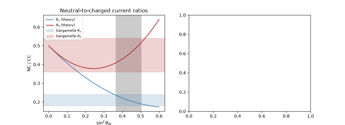
best fit sin^2 theta_W = 0.43, 1-sigma range 0.36 - 0.50
with no neutral currents, R_nu would be 0 (excluded by 7 standard deviations)

<matplotlib.legend.Legend object at 0x35003b3b0>

The single-electron event

\(\bar\nu_\mu e\to\bar\nu_\mu e\) can only happen through the \(Z^0\). Its cross section is proportional to \(g_L^2/3 + g_R^2\) (for \(\nu_\mu e\): \(g_L^2+g_R^2/3\)), with \(g_L=-\tfrac12+\sin^2\theta_W\), \(g_R=\sin^2\theta_W\). It is not small for any mixing angle, which is why a single clean event in the antineutrino film was so telling.

gL, gR = -0.5 + s2, s2
ax2.plot(s2, gL**2 + gR**2 / 3, color="steelblue", label=r"$\nu_\mu e$")
ax2.plot(s2, gL**2 / 3 + gR**2, color="firebrick", label=r"$\bar\nu_\mu e$")
ax2.axvspan(allowed.min(), allowed.max(), color="0.8", zorder=0)
ax2.set_xlabel(r"$\sin^2\theta_W$")
ax2.set_ylabel(r"$\sigma / (G_F^2 m_e E_\nu / \pi)$ (relative)")
ax2.set_title("Neutrino-electron scattering via the $Z^0$")
ax2.legend(fontsize=8)
fig.tight_layout()

plt.show()

Check

The Llewellyn Smith ratio: subtracting missed muons recovers R_nu; the data favour sin^2(theta_W) ~ 0.4, and R_nu = 0 (no neutral currents) is far excluded.

assert abs(R_corr - R_nu(s2_true)) < 3 * np.sqrt(R_nu(s2_true) / n_muon)
assert 0.3 < best < 0.5 and allowed.min() < 0.38 < allowed.max()
assert R_nu_obs / R_nu_err > 5