Asymptotic freedom and confinement: a receding quark pair’s string

Gross, Wilczek, and Politzer (1973) showed that the strong coupling decreases at short distances (asymptotic freedom), the opposite of QED – and, at long distances, lattice QCD (systematized by Wilson, 1974) confirms the coupling grows enough to confine quarks permanently inside color-neutral hadrons, via a linear potential \(V(r)=\kappa r\) at large separation. 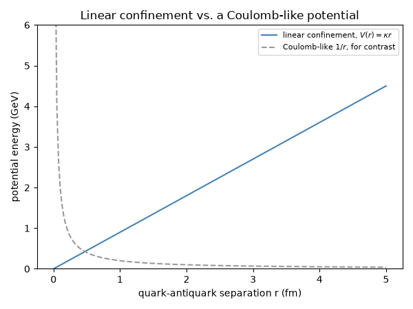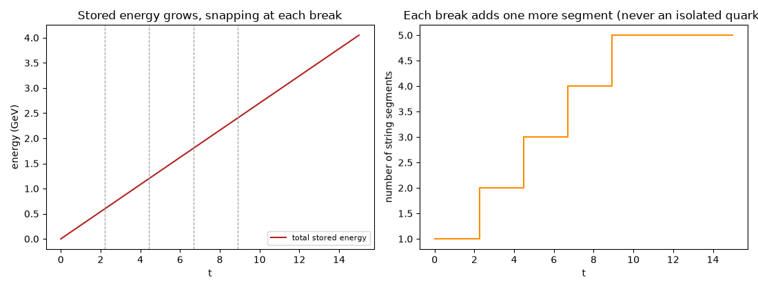This example evolves a receding quark-antiquark pair with string_break_chain(): the confining string’s stored energy, string_tension_energy(), grows without bound as the quarks separate – unlike a Coulomb-like potential that would let them escape to infinity – until it exceeds the threshold to pair-produce a new light quark-antiquark pair from the vacuum and the string breaks, repeatedly, rather than ever freeing a single isolated quark.

import matplotlib.pyplot as plt
import numpy as np

from physicskit.particle.confinement import string_break_chain, string_tension_energy
from physicskit.particle.visualizers import animate_string_breaking

Linear confinement: stored energy grows without bound

Unlike a Coulomb potential (~1/r, which lets two charges separate to infinity at finite cost), a linear potential’s stored energy grows without bound – exactly what forces the string to break rather than let an isolated quark escape.

kappa = 0.9  # GeV/fm, the standard lattice-QCD string tension
r_values = np.linspace(0.0, 5.0, 200)
energy = string_tension_energy(r_values, kappa)

fig1, ax1 = plt.subplots(figsize=(6, 4.5))
ax1.plot(r_values, energy, color="steelblue", label=r"linear confinement, $V(r)=\kappa r$")
ax1.plot(r_values[1:], 0.2 / r_values[1:], "--", color="0.6", label=r"Coulomb-like $1/r$, for contrast")
ax1.set_xlabel("quark-antiquark separation r (fm)")
ax1.set_ylabel("potential energy (GeV)")
ax1.set_title("Linear confinement vs. a Coulomb-like potential")
ax1.legend(fontsize=8)
ax1.set_ylim(0, 6)
fig1.tight_layout()

A receding pair: the string stretches, then breaks

v = 0.3  # recession speed, natural units
m_q = 0.3  # GeV, a light constituent quark mass (pair-production threshold 2*m_q)
t = np.linspace(0.0, 15.0, 400)
sim = string_break_chain(t, v, kappa, m_q, n_breaks=4)

print(f"string tension kappa={kappa} GeV/fm, recession speed v={v}c, light-quark mass m_q={m_q} GeV")
print(f"break times (when each successive break occurs): {np.round(sim['break_times'], 4)}")
print(f"segment extent at breaking, r_break_unit = 2*m_q/kappa: {sim['r_break_unit']:.4f} fm")

fig2, (ax2, ax3) = plt.subplots(1, 2, figsize=(11, 4.2))
ax2.plot(sim["t"], sim["energy_total"], color="firebrick", label="total stored energy")
for bt in sim["break_times"]:
    ax2.axvline(bt, color="0.6", ls="--", lw=0.8)
ax2.set_xlabel("t")
ax2.set_ylabel("energy (GeV)")
ax2.set_title("Stored energy grows, snapping at each break")
ax2.legend(fontsize=8)

ax3.step(sim["t"], sim["n_segments"], where="post", color="darkorange")
ax3.set_xlabel("t")
ax3.set_ylabel("number of string segments")
ax3.set_title("Each break adds one more segment (never an isolated quark)")
fig2.tight_layout()

string tension kappa=0.9 GeV/fm, recession speed v=0.3c, light-quark mass m_q=0.3 GeV
break times (when each successive break occurs): [2.2222 4.4444 6.6667 8.8889]
segment extent at breaking, r_break_unit = 2*m_q/kappa: 0.6667 fm

The breaking string, animated

anim = animate_string_breaking(sim)

plt.show()