Wilson’s lattice gauge theory: Wilson loops and the confining area law

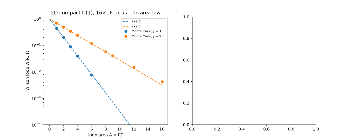
Wilson (1974) put gauge fields on the links of a space-time lattice and proposed a test for confinement: if large Wilson loops decay with the area they enclose, \(W(R,T) \sim e^{-\sigma RT}\), the static potential grows linearly, \(V(R) = \sigma R\), and charges cannot be separated. U1LatticeGauge samples compact U(1) gauge theory by Monte Carlo. In two dimensions the theory is exactly solvable (u1_2d_wilson_loop_exact()), so the measured area law and string tension can be checked exactly.

import matplotlib.pyplot as plt
import numpy as np
from scipy.special import iv

from physicskit.particle.lattice_gauge import (
    U1LatticeGauge,
    creutz_ratio,
    u1_2d_string_tension,
    u1_2d_wilson_loop_exact,
)

L = 16
loops = [(R, T) for R in range(1, 5) for T in range(R, 5)]

Monte Carlo Wilson loops against the exact solution

\(\ln W\) falls linearly with the loop area \(A = RT\), not with its perimeter: squares and elongated rectangles of equal area agree.

fig, axes = plt.subplots(1, 2, figsize=(12, 4.8))
sigma_mc = {}
for beta, color in ((1.0, "C0"), (2.0, "C1")):
    lat = U1LatticeGauge(L=L, beta=beta, seed=7)
    lat.thermalize(300)
    m = lat.measure(loops, n_measurements=1500, sweeps_between=3)
    A = np.array([R * T for R, T in loops])
    W = np.array([m[k][0] for k in loops])
    dW = np.array([m[k][1] for k in loops])
    ok = W > 3 * dW  # drop loops lost in statistical noise
    axes[0].errorbar(A[ok], W[ok], dW[ok], fmt="o", color=color, label=rf"Monte Carlo, $\beta = {beta}$")
    A_line = np.arange(0, 17)
    axes[0].semilogy(A_line, u1_2d_wilson_loop_exact(beta, A_line, volume=L * L), "--", color=color, label="exact")
    sigma_mc[beta] = creutz_ratio(m, 2, 2)
axes[0].set_yscale("log")
axes[0].set_ylim(1e-4, 1.2)
axes[0].set_xlabel("loop area A = RT")
axes[0].set_ylabel("Wilson loop W(R, T)")
axes[0].set_title(f"2D compact U(1), {L}×{L} torus: the area law")
axes[0].legend(fontsize=8)

<matplotlib.legend.Legend object at 0x16a9bcbf0>

String tension at every coupling

In 2D the string tension \(\sigma(\beta) = -\ln[I_1(\beta)/I_0(\beta)]\) is nonzero for every \(\beta\): U(1) charges are always confined, with \(\sigma \approx 1/(2\beta)\) at weak coupling. Creutz ratios \(\chi(2,2)\) from the simulations estimate it.

betas = np.linspace(0.2, 4, 100)
axes[1].plot(betas, [u1_2d_string_tension(b) for b in betas], "k-", label=r"exact $-\ln(I_1/I_0)$")
axes[1].plot(betas, 1 / (2 * betas), "k:", label=r"weak coupling $1/2\beta$")
axes[1].plot(list(sigma_mc), list(sigma_mc.values()), "s", ms=9, color="C3", label=r"Creutz ratio $\chi(2,2)$")
axes[1].set_ylim(0, 2)
axes[1].set_xlabel(r"$\beta = 1/g^2$")
axes[1].set_ylabel(r"string tension $\sigma a^2$")
axes[1].set_title("Confinement at all couplings in 2D")
axes[1].legend(fontsize=8)
fig.tight_layout()
for beta, s in sigma_mc.items():
    print(f"beta = {beta}: Creutz chi(2,2) = {s:.3f}, exact sigma = {u1_2d_string_tension(beta):.3f}")

beta = 1.0: Creutz chi(2,2) = 0.820, exact sigma = 0.807
beta = 2.0: Creutz chi(2,2) = 0.351, exact sigma = 0.360

A thermalized gauge field

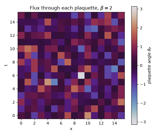
The plaquette angles \(\theta_P\) of one Monte Carlo configuration: random, uncorrelated flux, the disorder behind the area law.

lat = U1LatticeGauge(L=L, beta=2.0, seed=3)
lat.thermalize(200)
th = lat.theta.reshape(2, L, L)
theta_P = th[0] + np.roll(th[1], -1, axis=0) - np.roll(th[0], -1, axis=1) - th[1]
theta_P = np.angle(np.exp(1j * theta_P))
fig2, ax2 = plt.subplots(figsize=(5.5, 4.8))
im = ax2.imshow(theta_P.T, origin="lower", cmap="twilight", vmin=-np.pi, vmax=np.pi)
fig2.colorbar(im, ax=ax2, label=r"plaquette angle $\theta_P$")
ax2.set_xlabel("x")
ax2.set_ylabel("t")
ax2.set_title(r"Flux through each plaquette, $\beta = 2$")
fig2.tight_layout()

Check

2D U(1) lattice gauge theory confines at every coupling: the Creutz ratio gives the exact string tension -ln(I_1(beta) / I_0(beta)).

for beta, s in sigma_mc.items():
    assert abs(u1_2d_string_tension(beta) + np.log(iv(1, beta) / iv(0, beta))) < 1e-12
    assert abs(s / u1_2d_string_tension(beta) - 1) < 0.05