The November Revolution: discovery of the J/psi

In November 1974 two groups announced the same particle. Ting’s group at Brookhaven saw a sharp peak at 3.1 GeV in the invariant mass of electron-positron pairs from protons hitting beryllium. Richter’s group at SLAC tuned the SPEAR electron-positron collider across 3.1 GeV and saw the hadron production rate jump a hundredfold within a few MeV.

What made it revolutionary was the width. Hadronic resonances at this mass were expected to be hundreds of MeV wide; the J/psi is 93 keV wide, so it lives a thousand times longer than it “should”. The explanation was a new quark, charm, bound to its own antiquark and unable to decay by the easy routes. This example reproduces both measurements: the SPEAR energy scan, where the observed width is only the beam’s energy spread but the peak area still gives the true coupling, and the Brookhaven invariant-mass peak, built with two_body_decay() and invariant_mass().

import matplotlib.pyplot as plt
import numpy as np
from scipy.integrate import trapezoid

from physicskit.particle.decays import two_body_decay
from physicskit.particle.kinematics import FourVector, boost_generic, invariant_mass

M, Gamma = 3.0969, 93e-6  # GeV
Gamma_ee, B_had = 5.5e-6, 0.877  # GeV, hadronic branching fraction
HBARC2_NB = 0.3894e6  # (hbar c)^2 in nb GeV^2

SPEAR: scanning the beam energy

The Breit-Wigner cross section for \(e^+e^-\to J/\psi\to\) hadrons,

\[\sigma(E) = \frac{12\pi}{M^2}\, \frac{\Gamma_{ee}\Gamma_h/4}{(E-M)^2+\Gamma^2/4},\]

peaks near 80 microbarns but is only 93 keV wide, much narrower than the beams’ ~1 MeV energy spread. What the scan records is that peak smeared by the spread, sitting on a 20 nb continuum.

E = np.linspace(M - 0.012, M + 0.012, 24001)
sigma_bw = 12 * np.pi / M**2 * Gamma_ee * B_had * Gamma / 4 / ((E - M) ** 2 + Gamma**2 / 4) * HBARC2_NB
spread = 0.9e-3
kernel = np.exp(-0.5 * ((E - E.mean()) / spread) ** 2)
kernel /= kernel.sum()
sigma_obs = np.convolve(sigma_bw, kernel, mode="same") + 20.0

E_scan = np.linspace(M - 0.008, M + 0.008, 25)
rng = np.random.default_rng(1974)
sigma_scan = np.interp(E_scan, E, sigma_obs)
sigma_meas = sigma_scan * (1 + 0.05 * rng.standard_normal(E_scan.size))
print(f"true peak cross section:     {sigma_bw.max():,.0f} nb over a {Gamma * 1e6:.0f} keV width")
print(f"observed (beam-smeared) peak: {sigma_obs.max():,.0f} nb over ~{2.355 * spread * 1e3:.1f} MeV")

# The area under the peak doesn't care about the beam spread:
# integral(sigma dE) = 6 pi^2 / M^2 * Gamma_ee * B_had.
area = trapezoid(sigma_obs - 20.0, E)
Gamma_ee_fit = area / (6 * np.pi**2 / M**2 * B_had * HBARC2_NB)
print(f"Gamma_ee from the peak area: {Gamma_ee_fit * 1e6:.2f} keV  (input {Gamma_ee * 1e6:.1f} keV)")

true peak cross section:     79,387 nb over a 93 keV width
observed (beam-smeared) peak: 4,955 nb over ~2.1 MeV
Gamma_ee from the peak area: 5.49 keV  (input 5.5 keV)

Brookhaven: an invariant-mass peak

\(p+\mathrm{Be}\to J/\psi+X\), \(J/\psi\to e^+e^-\). Each pair’s invariant mass, measured with 1% momentum resolution, piles up at 3.1 GeV above a falling background of unrelated pairs.

masses = []
for _ in range(600):
    e1, e2 = two_body_decay(M, 0.000511, 0.000511, rng.uniform(-1, 1), rng.uniform(0, 2 * np.pi))
    beta = rng.normal(0, 0.3, 3)
    beta *= min(1.0, 0.9 / np.linalg.norm(beta))
    measured = []
    for e in (boost_generic(e1, beta), boost_generic(e2, beta)):
        p = e.p_vec * (1 + 0.01 * rng.standard_normal())
        measured.append(FourVector(np.linalg.norm(p), *p))
    masses.append(invariant_mass(measured))
background = 2.5 + rng.exponential(0.6, 3000)
print(f"\nBrookhaven-style peak: {np.median(masses):.3f} GeV, observed width {np.std(masses) * 1e3:.0f} MeV (all resolution)")

fig, (ax1, ax2) = plt.subplots(1, 2, figsize=(11, 4))
ax1.semilogy((E - M) * 1e3, sigma_bw + 20.0, color="0.6", lw=1, label="true line shape (93 keV wide)")
ax1.semilogy((E - M) * 1e3, sigma_obs, color="firebrick", label="smeared by beam spread")
ax1.errorbar((E_scan - M) * 1e3, sigma_meas, yerr=0.05 * sigma_scan, fmt="o", color="k", ms=3, label="scan points")
ax1.set_xlim(-8, 8)
ax1.set_ylim(10, 1e5)
ax1.set_xlabel(r"$\sqrt{s} - 3.097$ GeV [MeV]")
ax1.set_ylabel(r"$\sigma(e^+e^-\to$ hadrons) [nb]")
ax1.set_title("SPEAR: a more than hundredfold jump")
ax1.legend(fontsize=8)
ax2.hist(np.concatenate([masses, background]), bins=70, range=(2.5, 4.0), color="steelblue", alpha=0.85)
ax2.set_xlabel(r"$m(e^+e^-)$ [GeV]")
ax2.set_ylabel("pairs")
ax2.set_title("Brookhaven: a narrow peak at 3.1 GeV")
fig.tight_layout()

plt.show()

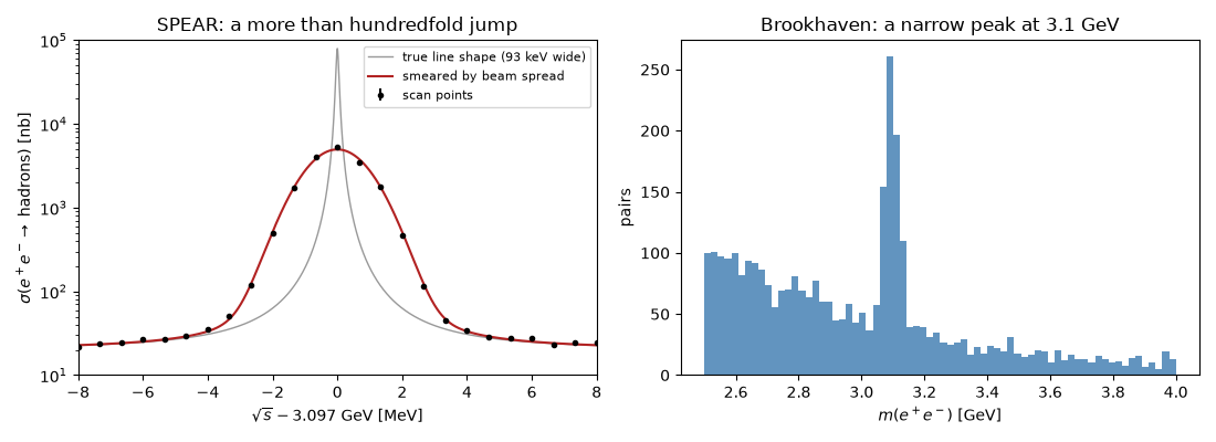
Brookhaven-style peak: 3.096 GeV, observed width 22 MeV (all resolution)

Check

Beam spread hides the 93 keV width but not the peak’s area, which gives Gamma_ee (Breit-Wigner); the dilepton mass peaks at 3.097 GeV.

assert abs(Gamma_ee_fit / Gamma_ee - 1) < 0.01
assert abs(np.median(masses) / M - 1) < 0.005
assert sigma_bw.max() > 10 * sigma_obs.max()