UA1 and UA2: discovery of the W and Z bosons

In 1983 CERN’s proton-antiproton collider, built on Rubbia’s proposal and van der Meer’s stochastic cooling, produced the carriers of the weak force for the first time. They were found in their decays to electrons.

The \(Z^0\to e^+e^-\) is an ordinary resonance: both electrons are measured, and their invariant mass (invariant_mass()) peaks at \(M_Z\). The \(W\to e\nu\) is harder, because the neutrino escapes and its momentum along the beam is unknown. Only its transverse momentum is inferred, from the imbalance of everything else seen. The trick is the transverse mass,

\[m_T = \sqrt{2\,p_T^e\,p_T^\nu\,(1-\cos\Delta\phi)} \le M_W,\]

whose distribution piles up just below a sharp edge at \(M_W\), the Jacobian peak. This example generates both decays with two_body_decay() and boost_generic() and extracts both masses.

import matplotlib.pyplot as plt
import numpy as np

from physicskit.particle.decays import two_body_decay
from physicskit.particle.kinematics import FourVector, boost_generic, invariant_mass

M_W, G_W, M_Z, G_Z = 80.4, 2.1, 91.19, 2.5
rng = np.random.default_rng(1983)


def produce(M, Gamma):
    """A boson with Breit-Wigner mass, a small pT and a longitudinal boost, decaying to two leptons."""
    m = M + 0.5 * Gamma * np.tan(np.pi * (rng.uniform() - 0.5))
    m = np.clip(m, M - 15, M + 15)
    l1, l2 = two_body_decay(m, 0.0, 0.0, rng.uniform(-1, 1), rng.uniform(0, 2 * np.pi))
    pT = rng.exponential(5.0)
    phi = rng.uniform(0, 2 * np.pi)
    pz = rng.normal(0, 60.0)
    E = np.sqrt(m**2 + pT**2 + pz**2)
    beta = np.array([pT * np.cos(phi), pT * np.sin(phi), pz]) / E
    return boost_generic(l1, beta), boost_generic(l2, beta)


def smear(lep, frac=0.03):
    p = lep.p_vec * (1 + frac * rng.standard_normal())
    return FourVector(np.linalg.norm(p), *p)

\(Z\to e^+e^-\): an invariant-mass peak

m_ee = np.array([invariant_mass([smear(a), smear(b)]) for a, b in (produce(M_Z, G_Z) for _ in range(2000))])
print(f"Z: median m(ee) = {np.median(m_ee):.2f} GeV  (input {M_Z})")

Z: median m(ee) = 91.16 GeV  (input 91.19)

\(W\to e\nu\): the transverse mass

The electron is measured (3%); the neutrino’s transverse momentum is the missing transverse momentum, with an extra 3 GeV of smearing from the rest of the event. Its longitudinal momentum is never used.

m_T, pT_e = [], []
for _ in range(8000):
    e, nu = produce(M_W, G_W)
    e = smear(e)
    nu_T = nu.p_vec[:2] + rng.normal(0, 3.0, 2)
    eT = e.p_vec[:2]
    cos_dphi = eT @ nu_T / (np.linalg.norm(eT) * np.linalg.norm(nu_T))
    m_T.append(np.sqrt(2 * np.linalg.norm(eT) * np.linalg.norm(nu_T) * (1 - cos_dphi)))
    pT_e.append(np.linalg.norm(eT))
m_T, pT_e = np.array(m_T), np.array(pT_e)

counts, edges = np.histogram(m_T, bins=80, range=(40, 100))
centres = 0.5 * (edges[1:] + edges[:-1])
smooth = np.convolve(counts, np.ones(3) / 3, mode="same")
print(f"W: m_T distribution peaks at {centres[np.argmax(smooth)]:.1f} GeV, just below M_W = {M_W} GeV")
print(f"W: fraction of events with m_T > M_W: {np.mean(m_T > M_W):.3f}  (only resolution and the W width leak past the edge)")
pt_counts, pt_edges = np.histogram(pT_e, bins=50, range=(10, 60))
print(f"W: electron pT distribution peaks at {0.5 * (pt_edges[np.argmax(pt_counts)] + pt_edges[np.argmax(pt_counts) + 1]):.1f} GeV  (M_W / 2 = {M_W / 2:.1f})")

fig, (ax1, ax2, ax3) = plt.subplots(1, 3, figsize=(15, 4))
ax1.hist(m_ee, bins=60, range=(70, 110), color="firebrick", alpha=0.85)
ax1.axvline(M_Z, color="k", ls="--")
ax1.set_xlabel(r"$m(e^+e^-)$ [GeV]")
ax1.set_ylabel("events")
ax1.set_title(r"$Z^0 \to e^+e^-$")
ax2.hist(m_T, bins=edges, color="steelblue", alpha=0.85)
ax2.axvline(M_W, color="k", ls="--", label=f"$M_W$ = {M_W} GeV")
ax2.set_xlabel(r"transverse mass $m_T$ [GeV]")
ax2.set_title(r"$W \to e\nu$: Jacobian edge at $M_W$")
ax2.legend(fontsize=8)
ax3.hist(pT_e, bins=60, range=(10, 60), color="darkorange", alpha=0.85)
ax3.axvline(M_W / 2, color="k", ls="--", label=r"$M_W/2$")
ax3.set_xlabel(r"electron $p_T$ [GeV]")
ax3.set_title(r"Electron $p_T$: Jacobian peak at $M_W/2$")
ax3.legend(fontsize=8)
fig.tight_layout()

plt.show()

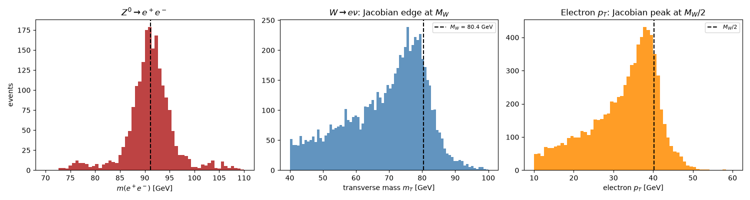
W: m_T distribution peaks at 78.6 GeV, just below M_W = 80.4 GeV
W: fraction of events with m_T > M_W: 0.138  (only resolution and the W width leak past the edge)
W: electron pT distribution peaks at 38.5 GeV  (M_W / 2 = 40.2)

Check

The Z is a dilepton peak at M_Z; the W shows a Jacobian edge in m_T at M_W and a Jacobian peak in the electron p_T near M_W / 2.

assert abs(np.median(m_ee) - M_Z) < 0.5
assert M_W - 4 < centres[np.argmax(smooth)] < M_W and np.mean(m_T > M_W) < 0.2
assert abs(0.5 * (pt_edges[np.argmax(pt_counts)] + pt_edges[np.argmax(pt_counts) + 1]) - M_W / 2) < 3