ATLAS and CMS: discovery of the Higgs boson

On 4 July 2012 ATLAS and CMS each reported a new boson near 125 GeV at five standard deviations. The cleanest channel was \(H\to\gamma\gamma\): a rare decay (0.2%) but one where both photons are measured precisely, giving a narrow peak in the diphoton invariant mass. It sits on a smooth, steeply falling background of ordinary photon pairs more than ten times larger under the peak.

Finding it is a question of statistics. This example builds signal photon pairs with two_body_decay(), boost_generic() and invariant_mass(), adds an exponential background, fits the background shape from the sidebands away from 125 GeV, and fits the signal strength with a binned Poisson likelihood. The local significance \(Z=\sqrt{2\,\Delta\ln L}\) grows as the square root of the collected data and crosses 5 sigma.

import matplotlib.pyplot as plt
import numpy as np
from scipy.optimize import minimize, minimize_scalar

from physicskit.particle.decays import two_body_decay
from physicskit.particle.kinematics import FourVector, boost_generic, invariant_mass

M_H = 125.1
rng = np.random.default_rng(2012)
bins = np.linspace(105, 160, 111)
centres = 0.5 * (bins[1:] + bins[:-1])


def diphoton_signal(n):
    """Reconstructed m_gammagamma for n Higgs decays, 1.2% photon energy resolution."""
    out = np.empty(n)
    for k in range(n):
        g1, g2 = two_body_decay(M_H, 0.0, 0.0, rng.uniform(-1, 1), rng.uniform(0, 2 * np.pi))
        beta = rng.normal(0, 0.35, 3)
        beta *= min(1.0, 0.9 / np.linalg.norm(beta))
        photons = []
        for g in (boost_generic(g1, beta), boost_generic(g2, beta)):
            E = g.E * (1 + 0.012 * rng.standard_normal())
            photons.append(FourVector(E, *(E * g.p_vec / g.p_mag)))
        out[k] = invariant_mass(photons)
    return out


def background(n, slope=0.035):
    u = rng.uniform(size=n)
    lo, hi = bins[0], bins[-1]
    return lo - np.log(1 - u * (1 - np.exp(-slope * (hi - lo)))) / slope


signal_pool = diphoton_signal(20000)
signal_shape = np.histogram(signal_pool, bins=bins)[0].astype(float)
signal_shape /= signal_shape.sum()
print(f"signal peak width (std of reconstructed mass): {np.std(signal_pool):.2f} GeV")


sideband = np.abs(centres - M_H) > 5


def poisson_nll(counts, lam):
    lam = np.clip(lam, 1e-9, None)
    return np.sum(lam - counts * np.log(lam))


def fit_background(counts):
    """Exponential fit to the sidebands (away from 125 GeV); returns b(m) in every bin."""
    x = centres - bins[0]
    res = minimize(
        lambda q: poisson_nll(counts[sideband], np.exp(q[0] - q[1] * x[sideband])),
        [np.log(counts[0] + 1), 0.03],
        method="Nelder-Mead",
    )
    return np.exp(res.x[0] - res.x[1] * x)


def significance(counts):
    """Signal strength and local significance, background fixed from the sidebands."""
    b = fit_background(counts)
    res = minimize_scalar(lambda mu: poisson_nll(counts, b + mu * signal_shape), bounds=(0, 5 * counts.sum() ** 0.5 * 10), method="bounded")
    Z = np.sqrt(max(2 * (poisson_nll(counts, b) - res.fun), 0.0))
    return Z, res.x, b

signal peak width (std of reconstructed mass): 1.07 GeV

Data sets of increasing size

One unit of luminosity holds 200 signal and 40,000 background events. Signal and background both grow in proportion to it. Any one data set fluctuates, so each luminosity is repeated in 25 pseudo-experiments; the median significance grows as \(\sqrt{L}\).

lumis = [0.5, 1, 2, 3, 4, 6]
Z_median, Z_lo, Z_hi = [], [], []
for L in lumis:
    Zs = []
    for _ in range(25):
        n_s = rng.poisson(200 * L)
        data = np.concatenate([rng.choice(signal_pool, n_s), background(rng.poisson(40000 * L))])
        counts = np.histogram(data, bins=bins)[0].astype(float)
        Zs.append(significance(counts)[0])
    Z_median.append(np.median(Zs))
    Z_lo.append(np.percentile(Zs, 16))
    Z_hi.append(np.percentile(Zs, 84))
    print(f"luminosity {L:>3}: median local significance {Z_median[-1]:.1f} sigma  (68% of experiments {Z_lo[-1]:.1f}-{Z_hi[-1]:.1f})")

fig, (ax1, ax2) = plt.subplots(1, 2, figsize=(11, 4))
counts = np.histogram(np.concatenate([rng.choice(signal_pool, 1200), background(240000)]), bins=bins)[0].astype(float)
ax1.errorbar(centres, counts, yerr=np.sqrt(counts), fmt="o", color="k", ms=2, lw=0.8, label="simulated data")
ax1.plot(centres, significance(counts)[2], color="steelblue", label="background fit (sidebands)")
ax1.axvline(M_H, color="firebrick", ls=":", label=f"$m_H$ = {M_H} GeV")
ax1.set_xlabel(r"$m_{\gamma\gamma}$ [GeV]")
ax1.set_ylabel("events / 0.5 GeV")
ax1.set_title(r"$H\to\gamma\gamma$: a small bump on a large background")
ax1.legend(fontsize=8)
ax2.fill_between(lumis, Z_lo, Z_hi, color="firebrick", alpha=0.2, label="68% of pseudo-experiments")
ax2.plot(lumis, Z_median, "o-", color="firebrick", label="median significance")
ax2.plot(lumis, Z_median[2] * np.sqrt(np.array(lumis) / lumis[2]), "--", color="0.5", label=r"$\propto\sqrt{L}$")
ax2.axhline(5, color="k", ls=":", label=r"5$\sigma$ discovery threshold")
ax2.set_xlabel("integrated luminosity (arbitrary units)")
ax2.set_ylabel(r"local significance [$\sigma$]")
ax2.set_title("Collecting data until the bump is a discovery")
ax2.legend(fontsize=8)
fig.tight_layout()

plt.show()

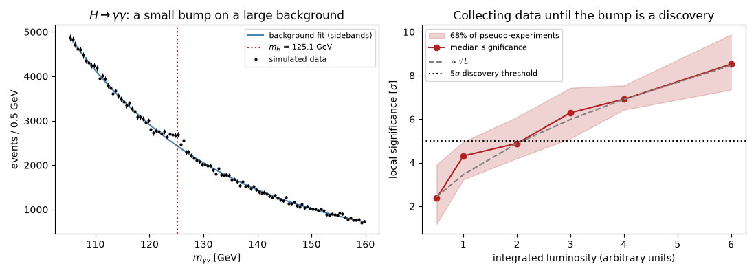
luminosity 0.5: median local significance 2.4 sigma  (68% of experiments 1.2-3.9)
luminosity   1: median local significance 4.3 sigma  (68% of experiments 3.2-5.0)
luminosity   2: median local significance 4.9 sigma  (68% of experiments 4.2-6.1)
luminosity   3: median local significance 6.3 sigma  (68% of experiments 5.1-7.4)
luminosity   4: median local significance 6.9 sigma  (68% of experiments 6.4-7.5)
luminosity   6: median local significance 8.5 sigma  (68% of experiments 7.3-9.9)

Check

The peak width is the photon resolution, 1.2% x M_H / sqrt(2); the median significance grows as sqrt(L) and passes 5 sigma within the scan.

assert abs(np.std(signal_pool) / (0.012 * M_H / np.sqrt(2)) - 1) < 0.15
assert abs(Z_median[-1] / (Z_median[2] * np.sqrt(lumis[-1] / lumis[2])) - 1) < 0.25
assert Z_median[0] < 5 < Z_median[-1]